How to Enter Formulas in Excel

This guide explains how to enter Formulas in Excel, with clear steps, practical tips, and important checks before you begin.

For the sake of convenience in the future, you should carefully study the following:

1. How to enter formulas starting with an equal sign.

To enter a formula in Excel, you must start with the equal sign or Excel will interpret it as a string. To enter the formula do the following:

Step 1: Type the equal sign at the position of the cell to calculate according to the formula.

Step 2: Enter the formula you want to calculate for that value cell.

Step 3: Press Enter to see results.

If you want to review the formula of that cell -> click on the cell position, the formula will show on the formula bar.

Example of calculating the total monthly revenue of the following enterprise:

- In the cell to calculate, enter the formula: = D6 + D7 + D8 + D9 + D10

- Press Enter -> the result is returned:

2. Learn about the formula of total values in a column.

With a formula that contains many terms if you simply use the plus sign -> it will take a lot of time and the results are incorrect -> you can use the formula function to calculate the total value in 1 column that Excel has supported.

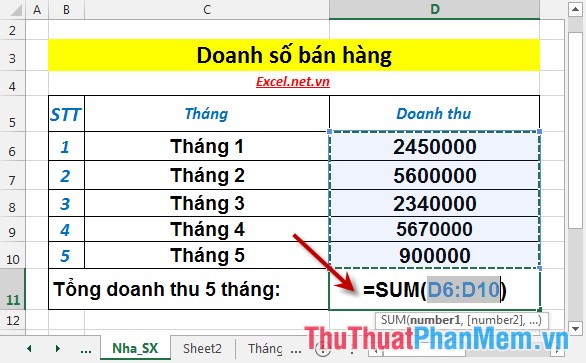
Step 1: Place the cursor at the position you want to sum -> Go to the Home tab -> Editing -> AutoSum -> Sum:

Step 2: Press Enter -> there is a formula in cell D11

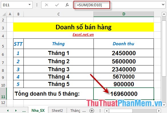
Step 3: Press Enter -> the result is:

3. Should copy a recipe instead of creating a new formula.

- In all special cases with a long complex formula, copying the formula is the best solution than creating a new formula. To copy the formula, follow these steps:

Step 1: Click the mouse on the cell containing the formula to copy -> move the mouse to the lower right corner of the cell until the mouse pointer changes to a dark dark cross:

Step 2: Hold down the left mouse button and drag the mouse to the bottom cell to be copied -> get the formula when the button appears Auto Fill Option button

Step 3: Revise the formula to suit the requirements.

- Where the cell containing the formula is not adjacent to the cell to copy the formula, you can use the key combination Ctrl + C and when pasting need to select a valid Paste style to maintain the old formula of the copied cell.

4. Learn about cells (cells) in Excel 2013.

In Excel to determine a cell based on the row index and the column index, in which the row index is numbered, alphabetically. Delivery of rows and columns is a cell, also known as a cell. Refer to description of cell:

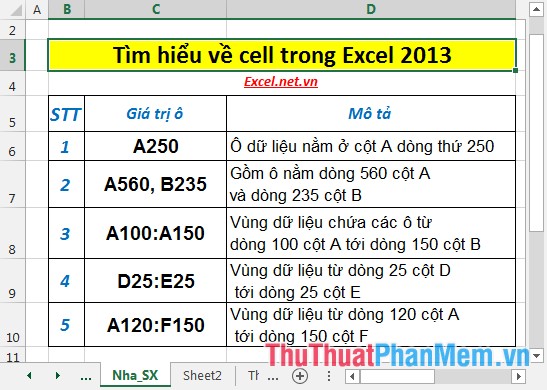
5. Update the results of the formula.

If you use a formula to calculate a series of data in cells, when there is a change in the value in cells -> the value in the formula automatically updates the changed value.

For example, the first 5 months of sales with the following data:

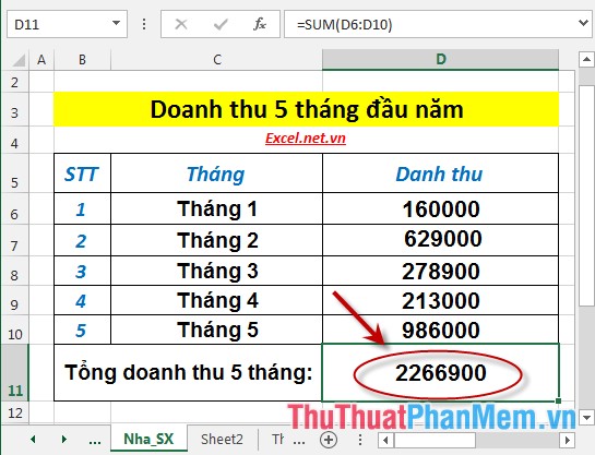
- In February, due to defective products returned by customers, the revenue decreased to 456700 -> revised February sales:

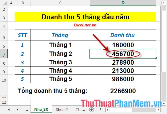
- Press Enter -> total sales in 5 months automatically updated according to the change of February revenue:

6. Use the Sum formula for several values in the column.

In case the values to be calculated are not contiguous -> you can use the following method and still use the Sum function:

For example, calculate the total turnover of the odd month:

Step 1: In the cell to calculate enter the formula: = SUM (D6, D8, D10). Note that each cell value in the column needs to be summed as a parameter of the Sum function and separated by commas:

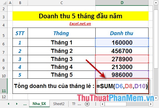
Step 2: Press Enter -> the result is:

7. Use other simple formulas in Excel 2013.

7.1 Calculate the average value.

Excel 2013 supports some simple calculation functions right in the toolbar. For example, let's quickly calculate the average turnover value of 5 months as follows:

Step 1: Click the mouse at the position you want to calculate the average value -> go to the Home tab -> Editing -> AutoSum -> Average.

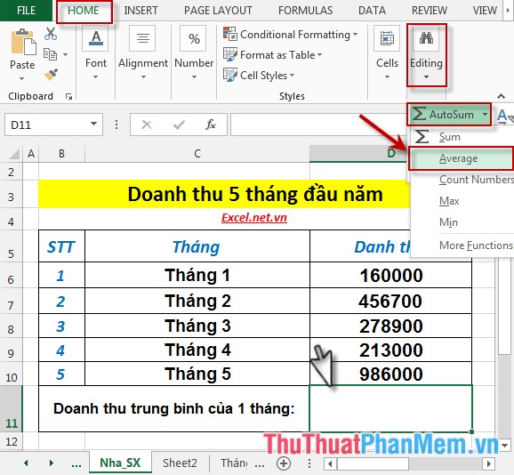
Step 2: After selecting Average the result is:

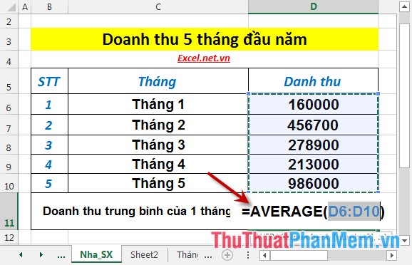
Step 3: Press Enter -> Average 5-month turnover is:

7.2 Find the maximum or minimum value.

- Similar to finding average value, maximum value or minimum value is the same. For example, find the biggest revenue in 5 months:

Step 1: Click the mouse at the position you want to calculate the maximum value -> go to the Home tab -> Editing -> AutoSum -> Max.

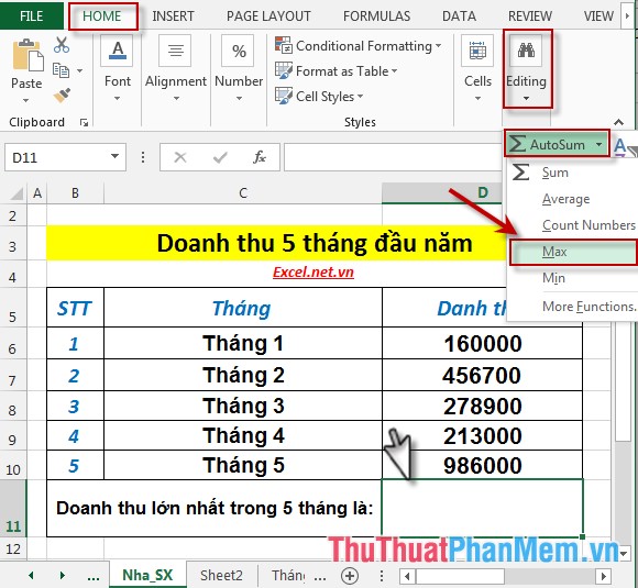
Step 2: Press Enter -> The biggest revenue in 5 months is:

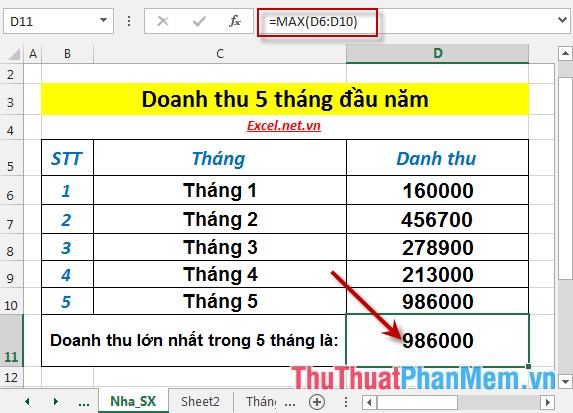
In the case of finding the smallest revenue, do the same instead of selecting Max to Min.

8. Print formulas for easy memorization.

If you need to memorize difficult formulas you can print them out so you can memorize them as quickly as possible. To do that you do the following:

- Condition: Your workbook must contain those formulas to be able to print.

- Conduct: Go to FORMULAS -> Formula Auditing -> Show Formulas.

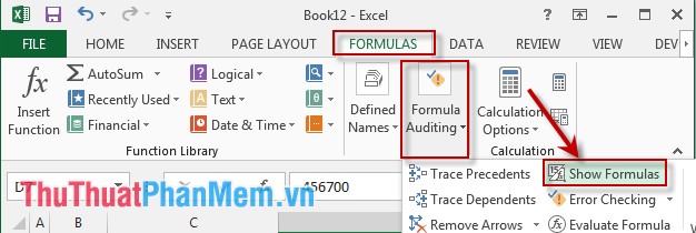
After clicking Show Formulas, all formulas in the workbook are displayed, you can print them normally:

9. Strange sign on the spreadsheet.

These are common mistakes and frequently encountered, please pay attention:

10. Learn other formulas.

- Excel supports many useful formulas for calculations. For more formulas, do the following: Go to Home -> Editing -> AutoSum -> More Function.

- A dialog box appears that you learn about other formulas in the Select Function section.

Above are instructions on how to enter formulas and some simple formulas that are frequently used in Excel 2013.

Good luck!