Instructions for creating interactive charts in Excel with INDEX function

Excel makes it easy to create clear, concise charts from your raw data.However, sometimes the graphs create static and not interesting.So the following article will introduce a simple method to help you turn static Excel charts into dynamic charts.

A simple drop-down menu (drop-down menu) can transform a simple Excel chart into an illustration image capable of presenting a variety of information and it's easy to set up.Here's how to use the INDEX function and the basic drop-down menu to create interactive charts in Excel.

Create data

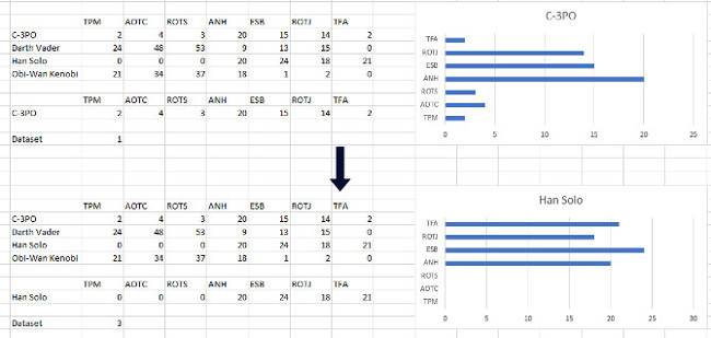
First thing to do is collect data.The image illustrated below is data about the time that appears on the screen of Star Wars movie characters.

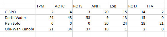
You just need to follow the steps similar to the following example with your metrics.Sort data by row, there is no space between them.When completing the chart, you can switch the position between C-3PO and Darth Vader and the chart will update with the correct data.

Next, copy and paste the title row below the data table.

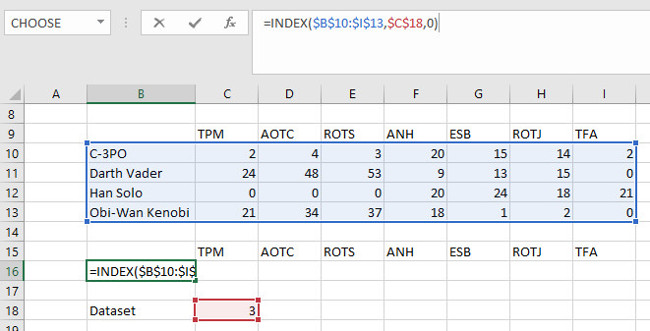
Now, in the third row from the title you just pasted, enter the word "Data" into a cell and enter a placeholder number in the box to the right next to it.From now on they will be placeholders as a basis for the drop-down menu.

When all is in place, we will join these elements with the INDEX function.Enter the following function formula on the two cells above theDataset:

 = INDEX ( $B $10 : $I $13 , $C $18 ,0 ) 

If you are new to using INDEX, let's analyze it.$ B $ 10: $ I $ 13 is the entire data that you want the formula to access, $ C $ 18 points to the cell that defines the display data (the number we put next to the Datasetcell).End the function with a column reference, but here we have specified the specific cell so the fill is 0.

The specifics of the function will vary depending on your data, so the image below shows the different components in the corresponding function on excel so you can do the same job.

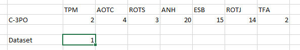
Only the arrow in the corner of the cell contains the function formula, you will see the arrow turn into a plus sign, then drag it out across the row.

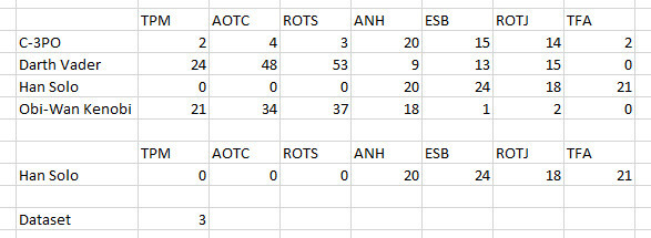
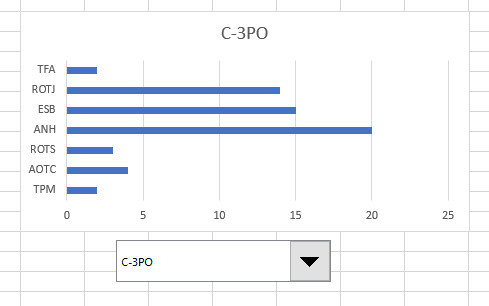
You will get the same results for the remaining cells as shown above.Now, you can manually change the number in the box to the right of theDataSet to use the INDEX formula. For example, enter 1in the box, the function will display data related to C-3PO.

Create a chart

Now the next step will be a little easier.We will choose the data we have after using the INDEX function - NOT the data that we enter manually - turn it into a chart.

To turn data into a chart, select Insert> Recommended Charts in the menu bar.

You can use any type of chart that best suits your data.In this example, the column chart seems most reasonable.

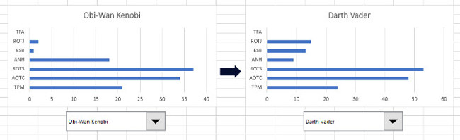
When the selection is complete, the graph showing the data will appear, test that everything is working by changing the number next to theDataSet.If the chart changes according to the data set you choose, then you have succeeded.

Add a drop down menu

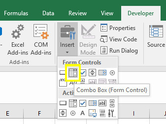
Now, make this animated graph a bit more "friendly".Select theDeveloper tab , click the Insert drop-down menu, in the Controls menu select Combo Box (Form Control).

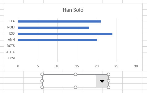
Create a drop-down menu wherever you want to place it but must be on the spreadsheet.In this example, the drop-down menu is located below the chart.

Right-click on the object and selectForm Control . Select the object for the data set in the Input rangefield.

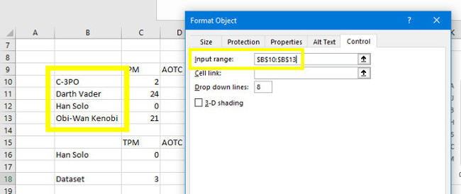
The Cell link field needs to match the cell containing the number indicating the selected data set.

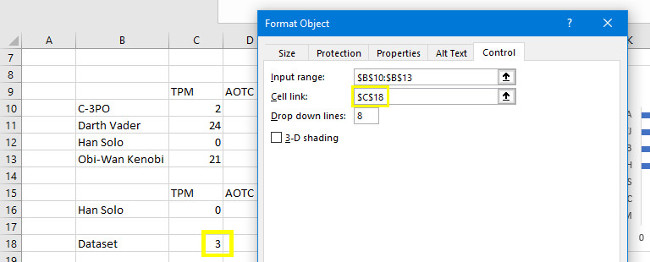
ClickOKand check the drop down menu.You will be able to select the data set by name and the chart will be updated automatically.

Once you're done, you can tweak the "look" to increase your spreadsheet's aesthetics, clean up some data to make the chart more compact.

For example, if you want to display all charts on the same page, copy and paste the chart, drop-down menu into a new worksheet.Then right-click on the drop-down menu and selectFormat Control.

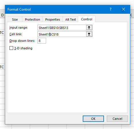
All you need to do is addSheet1! in front of the previously selected cell. This will tell Excel to find cells on a different sheet than the chart and drop-down menu. Click OKand we have a dynamic chart on a new, more neat and neat sheet.

So you can give yourself an interactive chart on Excel with INDEX function.Hope you find this article helpful and share it with the people around you.