How to use MAXIFS function in Excel 2016

What is MAXIFS function?

MAXIFS function in Excel is a statistical function that returns the largest value based on one or more conditions from the specified cells. MAXIFS function was introduced in MS Excel 2016.

Recipe

 = MAXIFS (max_range, criteria_range1, criteria1, [criteria_range2, criteria2], .) 

Argument:

1. Max_range (required argument) - The actual range of cells to which the maximum value will be determined.

2. Criteria_range (required argument) - The set of cells evaluated according to the criteria.

3. Criteria1 (mandatory argument) can be a numeric value, an expression or text that determines which cell will be rated as max.

4. Criteria_range2 - Optional argument in which an additional scope and their related criteria can be specified.

You can use up to 126 criteria.

How to use MAXIFS function in Excel

This is a built-in function that is used as a worksheet function in Excel. Consider some of the following examples:

Example 1:

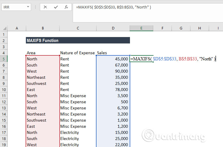
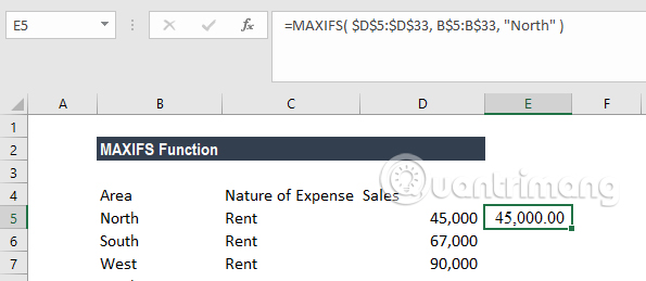
Suppose below is a table of quarterly revenue data for the three business areas. We will find the maximum revenue of the Northern region with the following formula:

 = MAXIFS ($ D $ 5: $ D $ 33, B $ 5: B $ 33, "North") 

In the above example, the MAXIFS function determines the rows with values ​​in column B equal to North and returns the largest value from the corresponding values ​​in column D.

Example 2:

In this example, we will find the area with the highest print and stationery sales with the following formula:

 = MAXIFS ($ D $ 5: $ D $ 33, C $ 5: C $ 33, "Printing & Stationary") 

The formula will return the highest amount of printing and stationery sales.

Example 3:

In this example, we will find the highest score for students earning Distinction scores for all subjects.

The formula will be:

 = MAXIFS (B6: B16, C6: C16, "A", E6: E16, "= Distinction") 

In criteria_range1, C10, C11 and C16 match the criterion 'A' of the corresponding cells in criteria_range2; E10, E11 and E16 satisfy Distinction criteria. Finally, the corresponding cells in max_range, B11 give the largest value. The result is 50.

Example 4:

With the data table below, we will use MAXIFS with the array function to return the latest date to open the task for each project in column E.

The formula is used as below:

For parentheses, we need to press Ctrl + Shift + Enter the first time because it only works as an array function. After that, we can drag it over the range to use.

Therefore, for the above data, we will see March 1, 2017 in Column F on all rows for Project A; 01/05/2017 for all rows of Project B; and 01/01/2017 for all rows of Project C.

Things to note about MAXIFS function

1. Error #VALUE! is returned when the size and shape of the max_range and criteria_rangeN arguments are not the same.

2. If you use an earlier version of Excel, you can use array functions based on MAX and IF to find the minimum value that meets the criteria.

3. #NAME? Error? occurs when using an older version of Excel (before Excel 2016).

4. MAXIFS will include hidden goods.

I wish you all success!

See more:

1. How to use the SWITCH function in Excel 2016
2. How to use the IFS function in Excel 2016
3. How to use the TEXTJOIN function in Excel 2016