How to use the TEXTJOIN function in Excel 2016

We are familiar with the CONCATENATE function to combine different strings or numbers in Excel. However it has some limitations:

1. Arguments must be separated by commas.

2. This function cannot retrieve the object in a scope to perform the merge.

3. It has no permissions to add separators.

With these disadvantages, a new function introduced in Excel 2016 is called TEXTJOINT, which performs the same function as CONCATENATE but is more efficient.

Description of TEXTJOIN function

The TEXTJOIN function concatenates text from multiple ranges and / or strings, which includes a delimiter between the connected text value. If the delimiter is an empty text string, this function effectively matches the ranges.

TEXTJOIN function syntax

This function has the following syntax:

 TEXTJOIN (delimiter, ignore_empty, text1, [text2], .) 

Let's parse the above:

1. Delimiter ( delimiter ) is the character inserted between the combined text. For example, a person's first and last name are combined with a '_' (underline) delimiter to identify the name easily and avoid spaces in the string. In this example, the underscore is a delimiter and the associated text is the first and last name.
2. Ignore empty is used to ignore empty cells while linking objects in scope. We can set options to ignore empty cells by leaving TRUE values ​​for this option and FALSE if we want to have empty cells.
3. Text 1 is the text to be combined, can be a single cell or a range of cells.
4. Text 2 is additional text that needs to be combined. You can use up to 252 text arguments, including Text 1. Similar to Text 1, it can be an individual cell or a range of cells.

Example of TEXTJOIN function

Here are some examples so you can better understand this function.

Example 1:

In this example, we have a data table that includes the names, surnames and states of each person. Here we will use the TEXTJOIN function to create a unique ID for each person by combining a first name, last name, and state. The formula uses an underscore as a delimiter, sets the second argument to TRUE so that there is no blank cell and range A2: C2 is the connected range.

How to use the TEXTJOIN function in Excel 2016 Picture 1

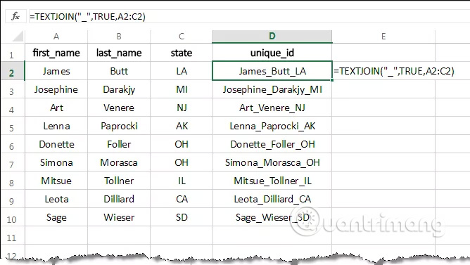
Drag the formula in cell D2 down, you will get the ID for each person.

Example 2:

In this example, still in the data table above, we find a list of all the names in the state of LA by using the TEXTJOIN function twice. First use the TEXTJOIN function in conjunction with the IF function to find out who matches the above condition, ie the person who lives in the LA state. The result will return the person's full name, when we pull down the formula, the column will be filled with their full name. If you live in another state, it will leave that box blank.

How to use the TEXTJOIN function in Excel 2016 Picture 2

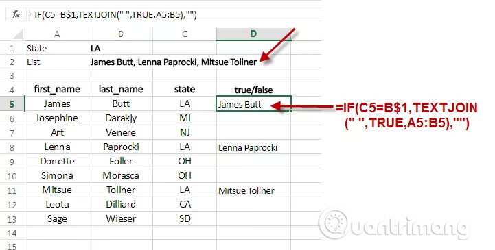
Next, we will use the TEXTJOIN function again to get the list in a comma separated by commas. To do so, we will write the following formula in cell B2.

 = TEXTJOIN (',', TRUE, D5: D13) 

As shown in the picture below:

How to use the TEXTJOIN function in Excel 2016 Picture 3

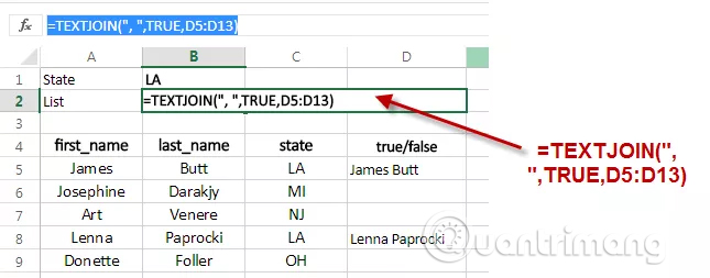
The result will be a comma-separated list of names as shown below:

How to use the TEXTJOIN function in Excel 2016 Picture 4

Empty cells will be ignored from the associated string because we set the second option to TRUE.

Example 3:

We can use the TEXTJOIN function to create auto-complete sentences. For example, use it to write a comment on a transcript to know which class it belongs to.

In the example below, we will create a LOOKUP table to find the student's corresponding class and return comments using the TEXTJOIN function. The following table contains point and class range information corresponding to that point range.

How to use the TEXTJOIN function in Excel 2016 Picture 5

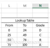
The LOOKUP formula is as follows:

 = LOOKUP (F4, L5: L8, N5: N8) 

As we know, LOOKUP has at least three arguments, first lookup value, F4 in this example. The second argument is the search range ie L5: L8 in this formula and the last argument is the returned range is N5: N8 in the formula. Therefore, the formula searches for points in the first column (Column L) and returns the value from Column N.

The formula for getting information from the following table is between E3: F5.

How to use the TEXTJOIN function in Excel 2016 Picture 6

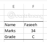
The Lookup formula is discussed in the preceding paragraph present in cell F5 and returns a C rank for 34. Now we will use the TEXTJOIN function to create a comment that can be placed in reports.

Suppose we want a sentence like this:

[Candidate tên] bạn có ký hiệu [ký hiệu], và bạn cấp là [Grade].

We will have the following formula:

 = TEXTJOIN ("", TRUE, F3, "You reached", F4, "points, ratings", F5, ".") 

In this formula:

1. The first argument is the delimiter that is set to a space (''), making it look like a sentence.

2. The second argument is set to TRUE as normal.

3. F3 is the name of the student

4. The sequel to 'You' will remain the same for each student's case.

5. Next is F4, points for students.

6. The next argument to the fixed section will remain the same for all cases.

7. The second argument is the class in cell F5.

8. The last argument is the punctuation expression ending the sentence.

I wish you all success!

See more:

1. These are the most basic functions in Excel that you need to understand
2. How to use Vlookup function in Excel
3. How to use the SUM function to calculate totals in Excel