How to name a cell or Excel data area

When you work with an Excel data sheet with multiple columns of information, the Define Name feature helps us name that column of information. This feature will help you name a cell, a data area or an array of data in an Excel table. When executing a formula, users can use the names of cells and direct ranges. If we move the named range, Excel will automatically update the formula with the named data area.

So the calculation of data on Excek will be faster and more accurate, the formula is shorter and easier to understand. The following article will guide you how to name the data area in Excel.

1. Guide to full Excel 2016 (Part 7): Format spreadsheet data
2. How to create duplicate data entry notifications on Excel
3. Instructions for searching and replacing in Excel tables

1. Instructions for naming a range of cells in Excel

Step 1:

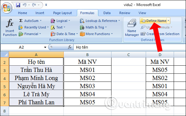
In the data table you are working click on the column you want to name and then select the Formulas tab in the toolbar, then select the Define Name as shown below.

How to name a cell or Excel data area Picture 1

Step 2:

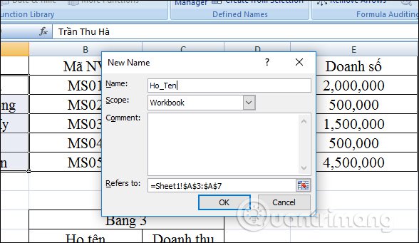
In the new dialog box that appears then there will be items to select content.

1. Name: Enter the name of the entry range. Name should be written immediately or with an underscore.
2. Scope: Range of ranges. Select Workbook if you want to apply to this Excel file or you can choose to apply it separately to 1 Sheet.

Click OK to set up.

How to name a cell or Excel data area Picture 2

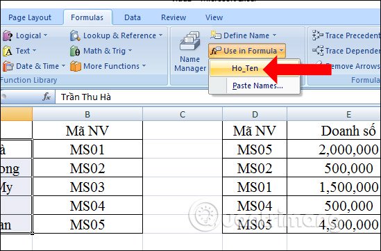
Then the set names will be in the Use in Formula section in the Formulas tab.

How to name a cell or Excel data area Picture 3

2. Name the ranges from an Excel data area

This way we will name multiple columns or multiple rows at once.

Step 1:

We select the cells we want to name for the whole range including the title, the title of the title will be the name of the sequence. Click on the Formulas tab and click on Create from Selection .

How to name a cell or Excel data area Picture 4

Step 2:

In the new dialog box interface, users will have more options:

1. Top row: Take the line above as the title.
2. Left Column: Take the left column as the title.
3. Bottom Row: Take the line below as the title.
4. Right Column: Take the right column as the title.

How to name a cell or Excel data area Picture 5

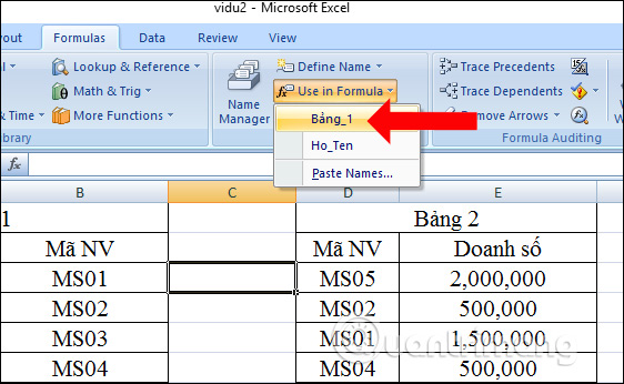
When we check, we will also see the data area name has been successfully set.

How to name a cell or Excel data area Picture 6

3. View and delete names that have been placed on Excel

To review the set names, click Use in Formula or Name Manager in the Formulas tab.

How to name a cell or Excel data area Picture 7

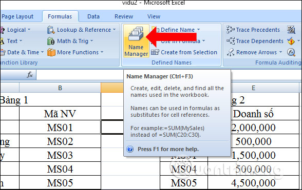
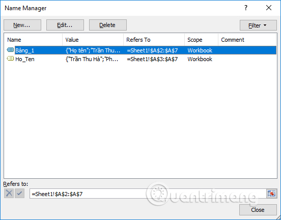
In case you want to delete, edit or create new content in the created range, click on Fromulas tab , select Name Manager . In the Name Manager interface box, click on the data set to create the name and the following options will appear.

1. New: Create a new name range.
2. Edit: Edit the content of the name sequence.
3. Delete: Delete the namespace.

How to name a cell or Excel data area Picture 8

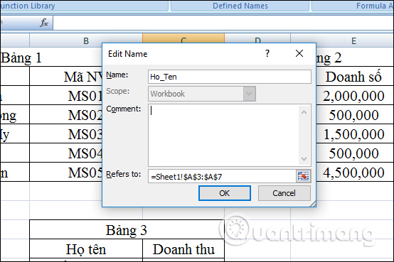
When clicking on the Edit item, users can change the set range name, select the named data area. In Scope alone, we cannot replace the scope of the range.

How to name a cell or Excel data area Picture 9

When you name the cells or data areas on Excecl, it is easier to remember the corresponding cell addresses. The implementation of the formula through the naming sequence is also faster. But users should note that the name must be less than 155 characters and do not use spaces, no symbols, except dots and underscores.

See more:

1. Create Excel charts that automatically update data with these three simple steps
2. 10 ways to recover corrupted Excel files
3. MS Excel - Lesson 4: Working with lines, columns, sheets

I wish you all success!