The way to color alternating columns in Excel is extremely simple

If you often have to work with a lot of data on Excel spreadsheets. At such times you need to be really focused because there are too many columns, many rows, and it's easy to get confused. To manage data more easily follow these steps:

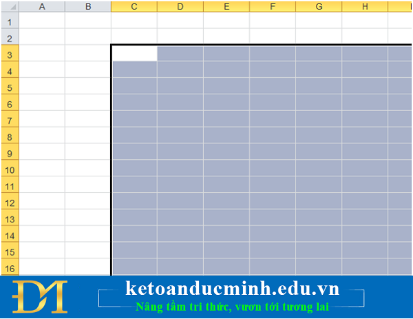
Step 1: Basic steps for coloring alternating columns in Excel

Drag and select the data columns to be colored, as in this example are from C3 to G16:

The way to color alternating columns in Excel is extremely simple Picture 1

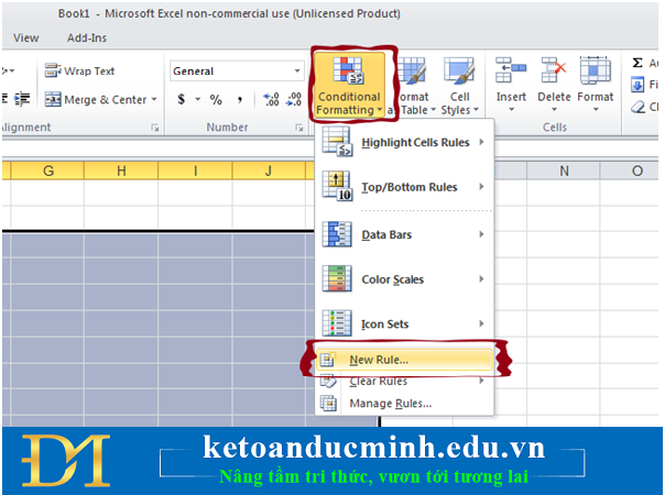
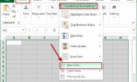
Step 2:

Select the Home menu> Condition Formatting> New Rule:

The way to color alternating columns in Excel is extremely simple Picture 2

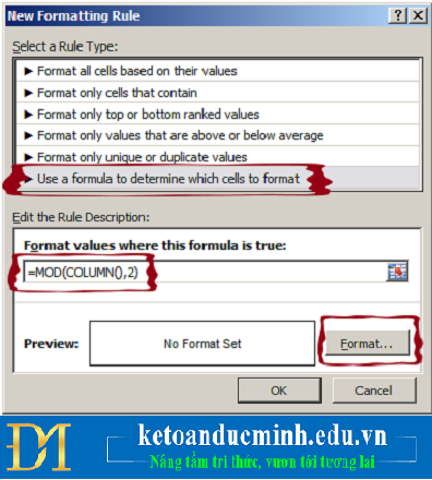
Step 3:

The New Rule table displays, select:

Use a Formula to dertermine which cells to format

At the box:

Format values ​​where this formula is true

We enter the formula:

= MOD (COLUMN (), 2)

Then choose Format to fill:

The way to color alternating columns in Excel is extremely simple Picture 3

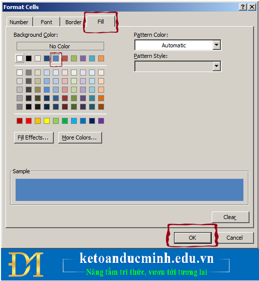
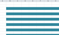
Step 4: Basic steps for coloring alternating columns in Excel

The Format Cells panel displays, select the Fill section as shown below. Select the color you want to fill in the different columns in the Background Color section, and then click the OK button:

The way to color alternating columns in Excel is extremely simple Picture 4

And here is our result:

The way to color alternating columns in Excel is extremely simple Picture 5

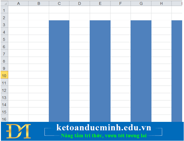
If you want the columns in the Excel worksheet to return to normal then you do the same as above, highlight the columns to select and then Home> Conditional Formatting> Clear Rule. The above is a simple trick to help us master Microsoft Excel spreadsheets more easily, avoid confusion when entering data, managing information.