Ways to hide data on Excel

In the Excel data sheet, there will be times when you need to hide some data to prevent others from seeing it. How to hide data on Excel is very simple and there are many different ways. We can easily hide or show Excel data again. Besides, users can still apply basic functions, calculation formulas in Excel to hidden data, without affecting the results or the whole data table.

The following article will summarize the ways to hide data on Excel to users, so that you can choose to match the Excel table being processed.

1. MS Excel - Lesson 4: Working with lines, columns, sheets
2. How to temporarily hide rows and columns in Excel 2013
3. Change color between different lines in Microsoft Excel

Method 1: Hide and show data by Checkbox

To hide or show data in columns or rows in Excel we have many ways to do it. The simple and manual way to hide Excel data is to press Unhide or Hide. However, this method is relatively manual and lacks professionalism. In case the content of long Excel documents you have to find the content to hide then proceed to hide or show again, relatively time consuming. If so, we can create a Checkbox to hide or display Excel data if needed.

1. Set up Checkbox on Excel

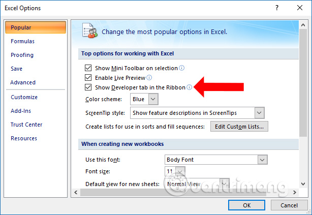
First, you need to display Developer mode on Excel to be able to use Checkbok. In Excel interface click on Office icon and select Excel Options. Display the new interface click on the Popular item and then look to the right to select Show Developer tab in the Ribbon .

Ways to hide data on Excel Picture 1

Step 1:

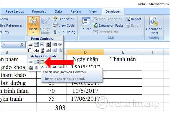
At the data interface in Excel, click on the Developer tab and then click Insert and select Checkbox . Select the location of the Checkbox box in Excel to make it easy to do. You draw the Checkbox in the position on the selected Excel.

Ways to hide data on Excel Picture 2

Step 2:

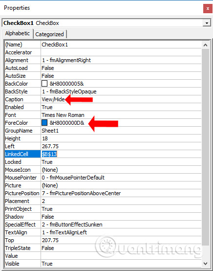
Next, click on Design Mode and select Checkbox on the content and click Properties in the interface. Or we can right-click on Checkbox and select Properties.

Ways to hide data on Excel Picture 3

This will display the new table interface for users to proceed to edit the content below.

1. Caption: Change the name Checkbox1 to View / Hide or whatever name you want.
2. LinkedCell: Enter any cell address like $ B $ 13. This box cannot be in the content content area to be hidden.
3. ForeColor: Change the font color on Checkbox.

Ways to hide data on Excel Picture 4

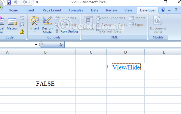
Turn off the Properties panel interface and click Design Mode again to remove the mode, which will show the value of the Checkbox box shown below. When you click on the Checkbox box, the value in cell B13 will change to TRUE.

Note that you must remove Design Mode to display TRUE and FALSE values ​​for Checkbox.

Ways to hide data on Excel Picture 5

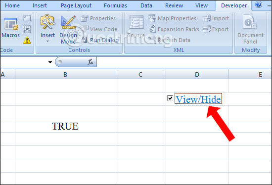
If you remove the check box in the Checkbox box, the value in cell B13 will become FALSE.

Ways to hide data on Excel Picture 6

2. Hide / show data by Checkbox

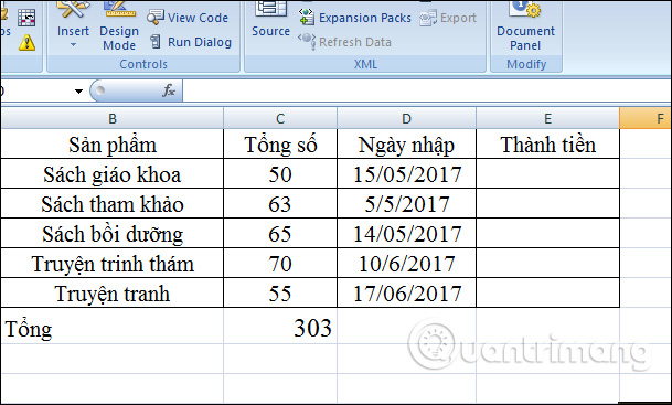
We will proceed to hide the Amount column in the data table below.

Ways to hide data on Excel Picture 7

Step 1:

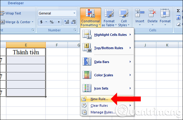
First you need to highlight the entire column of data you want to hide in Excel content, then click on the Home tab , select Conditional Formating and click New Rule .

Ways to hide data on Excel Picture 8

Step 2:

Displays the New Formating Rule dialog box. Here you find and click on the condition type to Use a formula to determine which cells to format in the list below. At the Format values line where this formulas is true enter the formula = $ B $ 13 = FALSE. Then click on the Format button next to it.

Ways to hide data on Excel Picture 9

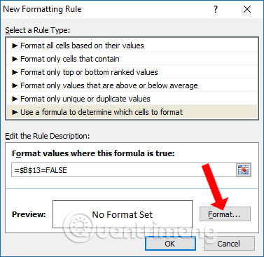
In the Format Cells dialog box click on the Font tab and then select the white for the font.

Ways to hide data on Excel Picture 10

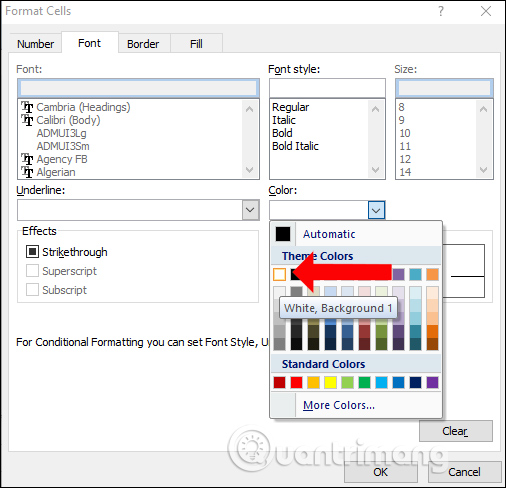
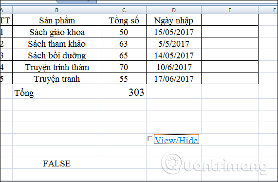
The result will be as shown below. When removing the check box in the View / Hide box, the value will change to FALSE, meaning that the data in the selected column will completely disappear.

Ways to hide data on Excel Picture 11

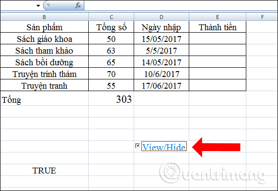
If the selected item is in the View / Hide box, the value will be converted to TRUE which means that the above column will automatically display the original content.

So if we want to hide the column or certain data area in Excel, we just need to tick, or leave the check box in the Checkbox box that has set the value to complete.

Ways to hide data on Excel Picture 12

Step 3:

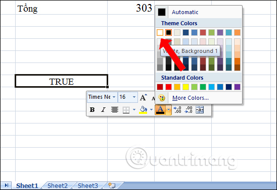
If you do not want to display TRUE or FALSE values ​​on Excel content, click on the value then switch to white text.

To remove the Checkbox in the content click on Design mode and then press the Delete key to delete.

Ways to hide data on Excel Picture 13

Method 2: Hide Excel data with Format Cells

Step 1:

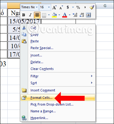
Black out the column to hide or the value to hide and right-click and choose Format Cells .

Ways to hide data on Excel Picture 14

Step 2:

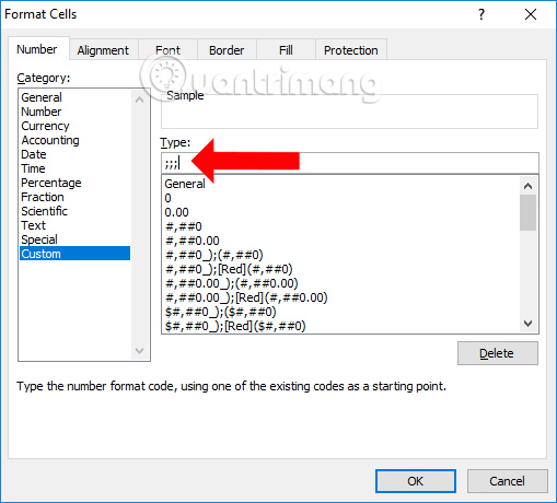
Switch to the new table interface, at the Number section, find the Custom option and look to the right in the Type section , enter 3 semicolons and click the OK button.

Ways to hide data on Excel Picture 15

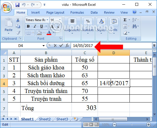
Back to Excel data table will see the value column has been hidden.

Ways to hide data on Excel Picture 16

Step 3:

To re-display the data in the column hidden in the data table, users can simply click on the hidden column is okay. If you click once, you will see the value in the top bar, and clicking twice will bring the data back to the table. Disabling the data will also disappear.

To show the data again, just remove 3 commas in the Format Cells table.

Ways to hide data on Excel Picture 17

Method 3: Hide Excel data by color

Step 1:

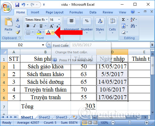
First, the user blackens the data area to be hidden and then clicks the letter A at the Home tab.

Ways to hide data on Excel Picture 18

Step 2:

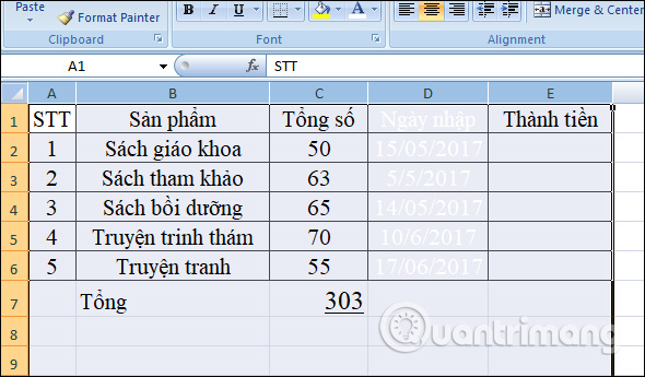
The user then just needs to switch the text to white to sync with the background color, or depending on which color depends on the data table background color.

Ways to hide data on Excel Picture 19

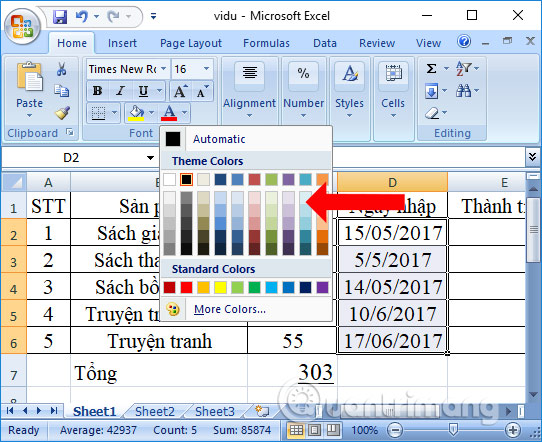
You will immediately see the data in the column completely hidden. If you want to show the data again, just change the text to black. However, this way of data is easy to see if blacked out. You only need to use this method temporarily.

Ways to hide data on Excel Picture 20

Method 4: Hide Excel data in the traditional way

We can immediately use the Hide / Unhide option for Excel columns to hide data. However, if you do this, the reader is very aware of which column is hidden, because the result will lose 1 column in the table.

Step 1:

You highlight the column to hide the data, then right-click and choose Hide to hide the data.

Ways to hide data on Excel Picture 21

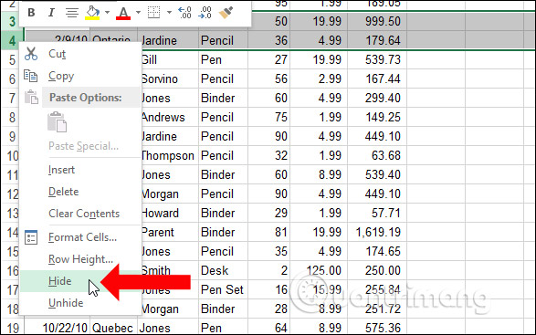
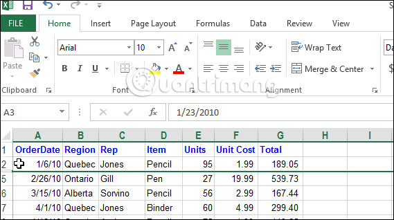
Immediately data in columns or rows in Excel will disappear.

Ways to hide data on Excel Picture 22

Step 2:

To display the hidden content in Excel, highlight the line, the column before or after the hidden content and press Unhide .

Ways to hide data on Excel Picture 23

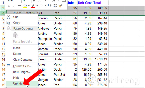
Note to readers , the Hide and Unhide options will only display in the right-click menu list with Excel 2010 or later. With the 2007 version, you have to pull it out.

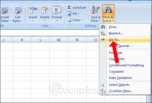
First, highlight the data column you want to hide and then click on the binoculars icon above to select Go to .

Ways to hide data on Excel Picture 24

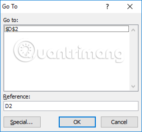
The table interface appears, here enter the column you want to hide data in Preferences then click OK.

Ways to hide data on Excel Picture 25

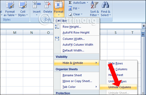
Back to the interface that still blackens the column you want to hide, click Format and then select Hide & Unhide and choose Hide Columns .

Ways to hide data on Excel Picture 26

To display the hidden content again, just highlight the table and click Format , select Hide & Unhide and select Unhide Columns .

Ways to hide data on Excel Picture 27

So you have 4 different ways to hide data, columns or rows in Excel tables. Each has different advantages and disadvantages. With the second way, changing the color for the data to hide in Excel is only applied temporarily.

See more:

1. How to hide files, show hidden files, view hidden folders and file extensions on Windows 7/8/10?
2. How to convert numbers into words in Excel?
3. How to change the default save file format in Word, Excel and Powerpoint 2016?

I wish you all success!