How to create List, Drop Down List in Excel

The following article shows how to create List, Drop Down List in Excel

1. Create a regular drop down list

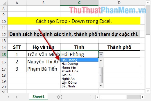
For example, there is a data field of provinces and cities, creating a drop down helps the data entry process be quick.

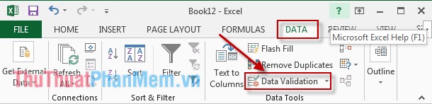
Step 1: Go to Data tab -> Data Validation .

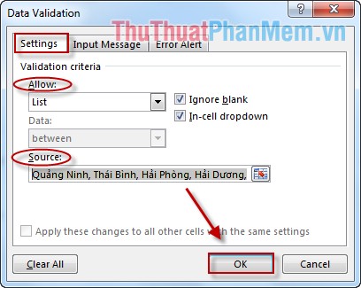
Step 2: The dialog box appears on the Settings tab in the Allow section select List , Source section enter the names of the components located in the drop down, the components separated by commas.

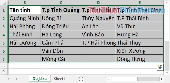
Alternatively you do not need to enter data directly, you can enter the components of the drop - down on another sheet. For example: Create a Du_Lieu sheet with the following provinces:

Click the icon -> move to Sheet Du_Lieu -> select all provinces:

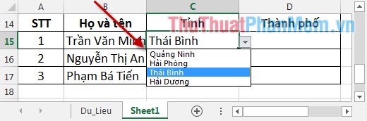
The results are the same as when created with direct input.

2. Creating a list depends on another list

For example: Enter the province list and city list depending on the province.

To create a dependent list, you should enter data into the list in the second way.

Step 1: Name the data regions.

Mandatory process of creating dependent lists you must name the relevant data areas:

+ The data area in the city of Quang Ninh province you highlight the data area from cell C2 -> cell C7 -> named QuangNinh (note the correct signs and capital letters, and do not contain space).

+ The data area from cell D2 -> cell D5 is named Hai Phong .

+ The data area from cell E2 -> cell E7 is named Thai Binh .

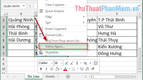
-> How to name as follows: Right-click on the data area you want to name -> Choose Define Name :

- A dialog box appears enter the corresponding name for the region as specified above:

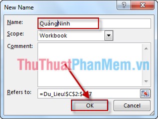
Please pay attention to the name so that it is the same as the value in the province name (but does not contain spaces).

Step 2: After naming the data, click on the cell to list -> Go to Data tab -> Data Validation .

Step 3: A dialog box appears in Allow, select List , Source in the following formula: = INDIRECT (SUBSTITUTE (C15, "", "")) .

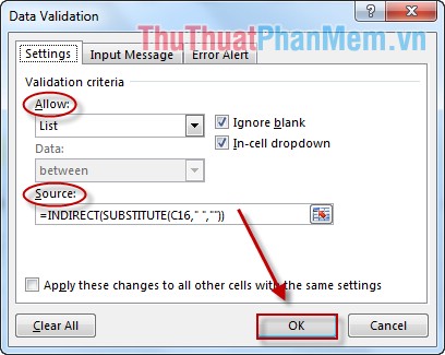
You notice in this step on the formula to the relative address otherwise the value between cities does not change.

Step 4: Click OK to get the results:

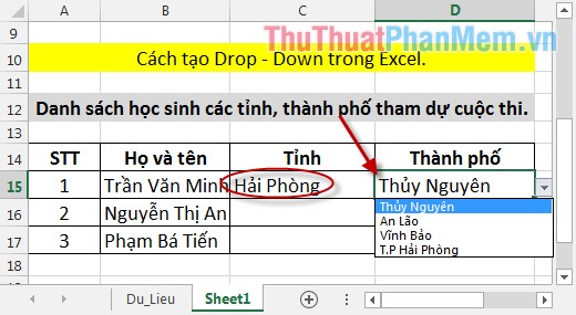
Similarly copy the formula for the remaining cells we have the results:

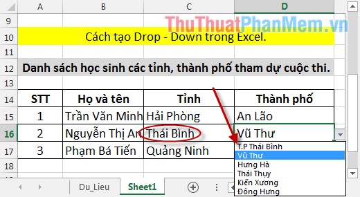
So you've created 1 list depends on another list. In this article, use the INDIRECT function in combination with the SUBSTITUTE function to get the value of the province name that has removed the space to refer to the data area with the same name as the reference value.

For example when the list provinces take the results of Thai Binh SUBSTITUTE perform delete spaces => reference value becomes thaibinh -> references the data area named thaibinh => The return value is the district in the province of Status Average from cell E2 -> cell E7 in the named data sheet.

Good luck!