How to create a drop list in Excel 2016

The drop-down list restricts the number of entries for an input field, avoiding spelling errors. Excel provides features to create flexible drop-down lists, so it is suitable for forms or data collection, making it easier for readers to select items in the drop-down list.

Use the drop-down list in a cell when there are specific options for that cell. For example, you can create a drop-down list containing options like Men and Women, Yes and No, etc. This article will show you how to create a drop-down list in Excel 2016 spreadsheet.

How to create a drop- down list in Excel

Here are the steps to create a drop-down list in Excel:

Step 1: Create a Range and name the data area: This step is necessary to create a user list for the drop-down list.

Step 2: Control input data with Data Validation : Data Validation feature displays a list of drop-down options or data type restrictions.

Step 3: Add the named data area to the Data Validation : Finally, add the data area to the Data Validation and specify the source for the drop-down list.

Step 4: Set the input message for Data Validation (optional): This step will add a message to guide users to use the spreadsheet.

Now, go to step-by-step details to create a drop-down list in Excel.

1. Create a data area

The way to add a list of items to a drop-down list uses Data Validation is to create a list in the spreadsheet and name the range containing the list. This list can be on the same worksheet or different worksheet as the drop-down list. Setting a priority for the range of cells in the drop-down list is easy for users to follow.

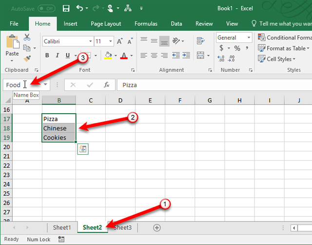
In this lesson, we will create a drop down list containing some different foods on Sheet 2 . Enter each item in a separate cell or in a column or row, then select items, name the selected range in the Name Box and press Enter .

1. Excel data entry faster

How to create a drop list in Excel 2016 Picture 1

2. Control input data with Data Validation

Go to the worksheet containing the drop-down list, click on the Data tab and then click Data Validation in the Data Tools section.

How to create a drop list in Excel 2016 Picture 2

3. Add the named data area to the Data Validation

In the Settings tab in the Data Validation dialog box, select List from the Allow drop-down list. We will use the name of the named range in the previous step , type the following in the Source box.

= Food

Replace "Food" with your data name, then click OK .

How to create a drop list in Excel 2016 Picture 3

Ignore blank is selected by default, it allows you to select a cell and then uncheck the box without selecting an item. If you want to select an option from the drop-down list, uncheck Ignore blank .

4. Set up data entry notifications for Data Validation

If you want to create a message displayed when selecting a cell in the drop-down list, click the Input Message tab, select the Show input message box when the cell is selected and fill in the Title and Input messages box. In addition, you can also use the Error Alert tab to add a message that appears when invalid entered in the drop-down list (for example, if someone typed in the box instead of selecting the option). Select Show Error alert after invalid data is entered , then select Style and fill in the Title and Error message box , click OK.

How to create a drop list in Excel 2016 Picture 4

The arrow appears only when the cell containing the drop-down list is selected and is located to the right of the cell. If the drop-down list contains more than eight items, you'll see a scroll bar in the drop-down list when clicking the arrow.

How to set the book to the top

Edit or delete a data area

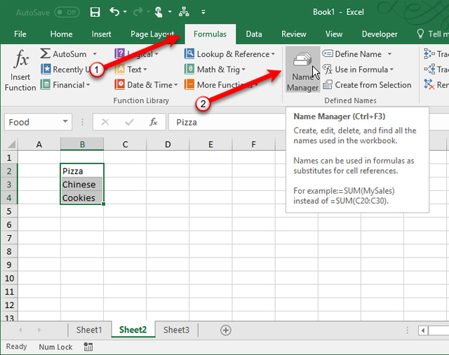
To edit or delete a named range, use Name Manager , click the Formulas tab, and then select Name Manager in the Defined Names section.

How to create a drop list in Excel 2016 Picture 5

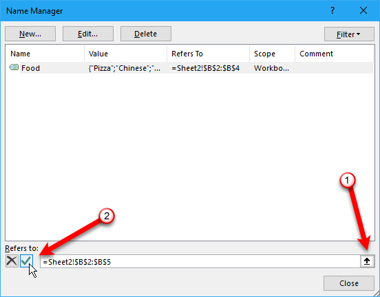
To change the range name in the Name Manager dialog box, select Name in the list and click the cell range button at the bottom of the dialog box. Then, select the range and click the umbrella button again in the thumbnail of the Name Manager dialog box. Next, click the green checkmark button to save the new range with the selected name.

How to create a drop list in Excel 2016 Picture 6

Alternatively, you can change the name by selecting it in the list, clicking Edit , changing the name in the Edit Name dialog box and clicking OK or changing the range of cells on the Edit Name dialog box . To delete a name, select Name in the list and click Delete .

Create a dependent drop-down list

The dependent drop-down list is a list of options that vary according to the options in the main drop-down list. For example, when selecting Pizza in the drop-down list, the second dependent drop-down list will contain pizza types. If you select Chinese, the options in the dependent drop-down list will contain different types of Chinese dishes.

Before starting, go back to the previously created drop-down list and create a Favorit Food drop-down list if you haven't already. Now we will create three more lists and name them. Enter a list for each option in the main drop-down list, then name that list in Name Box and press Enter . Do the same for the remaining listings.

The names of other lists must match the options in the main drop-down list. For example, the list contains cookies that will be named Cookies . The other two lists in the red box as shown below are named Pizza and Chinese .

How to create a drop list in Excel 2016 Picture 7

Before creating the dependent drop-down list, select an item in the main drop-down list. Then, select the cell you want to add the dependent drop-down list.

How to create a drop list in Excel 2016 Picture 8

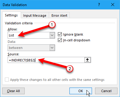
Click the Data tab and then click Data Validation in the Data Tools section. Select List in the Allow drop-down list . Enter the following text in the Source box, replace " $ B $ 2 " with a reference to the cell containing your main drop-down list, but remember to keep the dollar symbols in the cell reference, which is an absolute reference to that cell will not change even when copying or moving the reference formula to that cell.

1. These are the most basic functions in Excel that you need to understand

= INDIRECT ($ B $ 2)

INDIRECT returns the reference specified with a text string, in this case the text from the selected option in the main drop-down list in cell B2. For example, if you select Chinese from the main drop-down list, = INDIRECT ($ B $ 2) will return the Chinese reference. Therefore, the second drop-down list contains Chinese entries. Then, click OK .

How to create a drop list in Excel 2016 Picture 9

The list in the Favorite Dish drop-down list in the example below changes depending on the selection in the main Favorite Food drop-down list.  

How to create a drop list in Excel 2016 Picture 10

Copy and d projects the drop- down list

To copy the drop-down list with data control to other cells, press Ctrl + C and Ctrl + V on the cell you want to copy to copy the list and keep the format.

If you just want to copy the drop down list with data control but don't need to keep the format, select the cell you want to copy and press Ctrl + C , then go to the Home tab and click Paste in the Clipboard section, select Paste Special .

1. 10 ways to use the Paste feature in Excel

How to create a drop list in Excel 2016 Picture 11

On the Paste Special dialog box, select Validation in the Paste section, then click OK .

How to create a drop list in Excel 2016 Picture 12

Note: You must be very careful when working with the drop-down list in Excel. When copying a cell that does not contain a drop-down list to a cell that contains a drop-down list, this list will be lost. Excel does not display a notification about the operation, but you can still undo it by pressing Ctrl + Z.

Select all cells containing the drop- down list

Because the arrow button is not displayed on the drop-down list unless the cell is selected, it is difficult to know which cell contains the drop-down list. You can apply different formats to the cells in the drop-down list for easy distinction. But first you need to find all the drop-down lists. There is a way to select all the cells that contain the drop-down list. First, select a box containing the drop-down list, go to the Home tab and click on Find & Select in the Editing section, then select Go To Special .

How to create a drop list in Excel 2016 Picture 13

On the Go To Special dialog box, select Data Validation . All option under Data Validation will select all cells that apply data control rules. The Same option selects only the cells in the drop-down book using the same data control rules as the selected cell.

Select the option that fits your data, here select All because the drop-down list uses different rules, then click OK .

How to create a drop list in Excel 2016 Picture 14

Two drop-down lists are selected.

How to create a drop list in Excel 2016 Picture 15

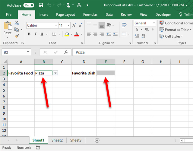
You can now format these cells to distinguish them from other cells.

The way to make an arrow in the drop-down list always appears

The arrow buttons on a drop-down list will disappear when no cells are selected. We will solve this problem by adding the arrow button permanently to the right of the drop-down list.

To create an arrow that always appears in the drop-down list, take a screenshot containing the arrow in the list, then take the arrow, insert the image into the box to the right of the drop-down list, so you will see Arrow button even if you don't select the drop-down list. When selecting the drop-down list, the arrow button will appear on the inserted image.

To start, download the drop-down-arrow.png arrow file (right-click on the link and select Save link as ). Then, select the box to the right of the drop-down list and go to the Insert tab.

How to create a drop list in Excel 2016 Picture 16

Click Illustrations and select Picture .

How to create a drop list in Excel 2016 Picture 17

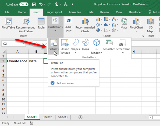
On the Insert Picture dialog box, navigate to the location of the downloaded file above and select the file, then click Insert .

How to create a drop list in Excel 2016 Picture 18

The image is inserted to the left of the cell.

How to create a drop list in Excel 2016 Picture 19

Delete a drop- down list in a cell

To delete the drop-down list in a cell, select that box and open the Data Validation dialog box (go to the Data tab and click Data Validation in the Data Tools section), click the Clear All button . The options on the Data Validation dialog will be set to the default value, then click OK .

How to create a drop list in Excel 2016 Picture 20

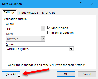
The drop-down list has been deleted and the box will be restored to its default format. If there is an option selected when deleting the drop-down list, that cell will be entered with the value of that option.

How to create a drop list in Excel 2016 Picture 21

If you don't want to save any value when deleting the drop-down list, you can copy the blank cell and paste it in the box that contains the drop-down list, which will be deleted.

See also: Summary of expensive shortcuts in Microsoft Excel