How to make Excel spreadsheets smarter with drop-down lists

Despite their power, they are often overlooked in Excel's user interface, causing many users to miss out on their benefits. Are you ready to make your spreadsheet smarter? Here's how you can use drop-down lists in Excel

How to create a drop-down list in Excel

Excel drop-down lists are properly classified in the Data Validation tab , as they not only streamline data entry but also enhance the reliability of formulas.

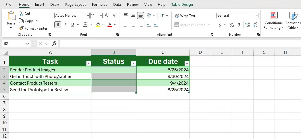
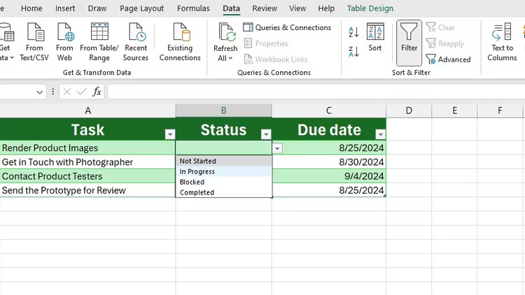
This example will use a task tracker with a Status column that provides a drop-down list for each task. List items will include Not Started, In Progress, Completed and Blocked.

Unlike Google Sheets, Excel requires list values ​​to exist somewhere in the workbook. To avoid cluttering the task tracker, it's best to create a separate sheet to store these values. After creating a drop-down list, you can hide cells or the entire worksheet to keep your tracker neat.

Here's how to set up a drop-down list:

1. Prepare your list values ​​by entering the list items (for example, Not Started, In Progress, Completed, Blocked) in a column on a separate worksheet.
2. Highlight the cells where you want the drop-down list to appear (for example, B2:B5).
3. Go to the Data tab on the ribbon, then click Data Validation in the Data Tools section .
4. In the Data Validation window, select List in the Allow drop-down list .
5. Click the up arrow in the Source field and select the range containing your list items.
6. Click OK to apply the drop-down list to the selected cells.

Selected cells will now display drop-down arrows, allowing you to choose from predefined items.

How to customize Excel drop-down list

Although the drop-down list is rich in functionality, it may not be as visually appealing as it should be, especially if you are used to colorful drop-down lists in Google Sheets. Luckily, with just a little Excel conditional formatting, you can improve the look of drop-down lists in Excel.

To apply conditional formatting to a drop-down list, follow these steps:

1. Highlight cells with drop-down lists (for example, B2:B5 ).
2. Go to the Home tab , click Conditional Formatting and select New Rule .
3. In the New Formatting Rule window , select Format only cells that contain .
4. In the rule description, set the first drop-down list to Specific Text and leave the second field as is.
5. Enter the text you want to format (for example, Completed).
6. Click Format next to the preview. In the Format Cells window , set the Font to white, go to the Fill tab , and choose a dark green color for the background.
7. Click OK twice to apply the rule.

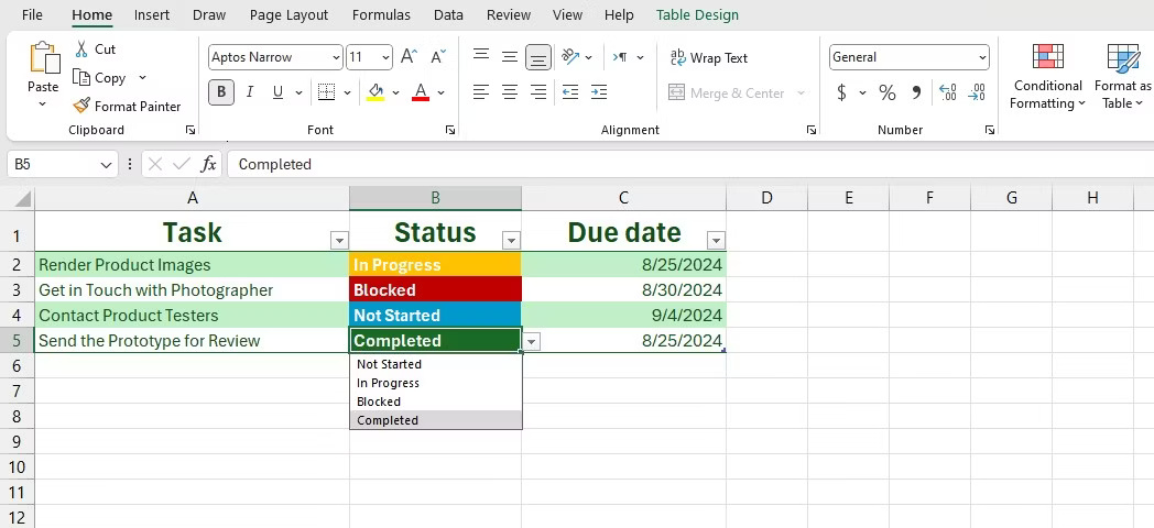
Now, any task marked as Completed will have a green background, making it easy to identify at a glance. Repeat these steps for the other list items and assign each item a unique color. This will greatly improve visual clarity.

The drop-down list eliminates the risk of typos and variations - no more Complete, Finished or Done. This consistency is important when analyzing data using formulas; For example, if a formula tracks completed tasks, the formula will miss tasks marked as Finished.

Now, with drop-down lists, your Excel spreadsheet is not only easier to use, but also prepared for advanced data analysis. You can filter tasks by status, such as showing only In Progress tasks, or use the COUNTIF function to count the number of blocked tasks.

Micah Soto

Update 27 August 2024