Calculate the subtotal of the list on Excel

Lists are new properties that are very useful in Excel 2003 if you don't want to calculate subtotals of columns; Excel always disables the Subtotal feature for the list. Currently, in order to manage the list and perform subtotal calculations, you will have to proceed in a very complicated way. So temporarily convert the list into a traditional format and make it easier to calculate subtotals.

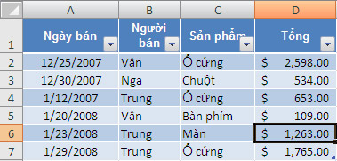
Excel 2007 calls lists as tables. If you are using a version of Excel 2002 or a previous version, you can still use the Subtotal feature. You will know where the lists are located with small controls that can drop down to the right of each cell title.

Table list in Excel

Before you can calculate subtotals of list data, you must convert to the regular list as follows:

1. Click your mouse anywhere on the worksheet.

2. For Excel 2003, select Lists from the Data menu and select Convert to Range . If you are using Excel 2007, click on the Design tab and click Convert to Range on the toolbar group.

3. Click OK .

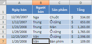
Table after having moved to the normal list

After converting the list into a regular format, please sort the data according to your computing needs. For example, to calculate the subtotal of the Total by Seller column, you must first sort the data by the Seller's column as follows:

1. Click your mouse anywhere on the Seller's column.

2. For Excel 2003 and earlier versions, click Sort Ascending or Sort Descending as required. For Excel 2007, you must sort in a special way by clicking Sort and Filter on the Home tab, selecting Custom Sort .

Arrange tables by Sellers group

After the group arrangement has been completed, you can start conducting subtotals by following these steps:

1. Place the mouse pointer anywhere on the spreadsheet.

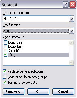
2. For Excel 2003, select Subtotals from the Data menu. If you are using Excel 2007, click Subtotal in the Outline group on the Data tab. In the Subtotal dialog box you have several options as follows:

1. At At Each Change In , select the column that calculates the subtotal (Not the column whose values ​​will count subtotals). In the example is the Seller column.
2. At Use Function , select the appropriate function. Sum is the default function and in the example Sum is the selected function.
3. Check the corresponding columns in the Add Subtotal To section section . In the example you select Total .

3. After determining the correct column and function, click OK .

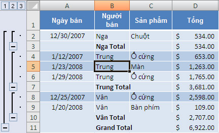
This feature will add a subtotaling row for each group that you defined on the Subtotals dialog window. In the above example, Seller is the group where Excel displays a subtotal.

To restore the previous list, select the worksheet and press Ctrl + L and click OK to close the Create List dialog box. You won't even have to delete the subtotal first. Even the first time you sort any list, Excel warns you that this subtotal will be deleted. However, you can delete the subtotals by displaying the Subtotal dialog window and clicking Remove All .