The use of the Split tool separates the Excel data table

Computer screen split feature supports users a lot in observing content, comparing content on different windows. With Excel, too, when you split the data table horizontally or vertically, you can see more of the worksheet without dragging too much. Especially if the user needs to compare the data in the long table, it can be split into different parts to check. To separate the data table in Excel, we need to use the Split tool on Excel and guided in the following article of Network Administrator.

1. How to keep Excel and Excel columns fixed?
2. Instructions for separating column content in Excel
3. How to separate sheets into separate Excel files
4. How to separate the date, month, and year columns into 3 different columns in Excel

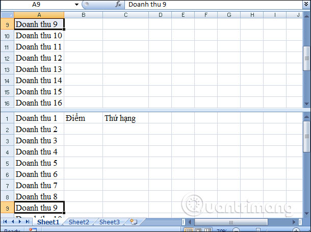
The use of Split splits the Excel table into 4

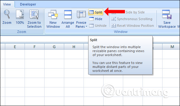
Step 1:

First click on cell A1 in the Excel data sheet and click on the View tab on the toolbar. Then select the Split feature .

The use of the Split tool separates the Excel data table Picture 1

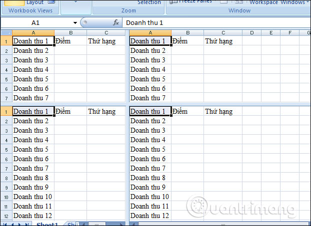
The result of Excel file has been split into 4 data tables as shown below. The content in each data sheet is the same.

The use of the Split tool separates the Excel data table Picture 2

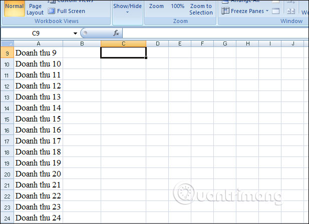
Step 2

4 data tables are evenly aligned and separated by 2 horizontal and vertical lines when you click. You can narrow or stretch the data table area, not leaving the center at the center depending on the need. Can be narrowed to the left or right depending on the user.

The use of the Split tool separates the Excel data table Picture 3

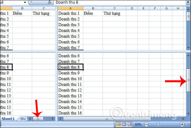
Step 3:

Each section of the data sheet has a scroll bar that moves up and down or left to right. Thus users can easily compare data in 4 tables. To cancel the separation of Excel table just press the Split feature again.

The use of the Split tool separates the Excel data table Picture 4

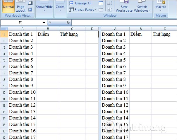
2. How to divide the Excel data table into 2 parts

If the user does not want to divide the above 4 sections, it is possible to divide the vertical or horizontal data tables into 2 data tables.

Step 1:

To separate the data table horizontally into 2 parts, users click on the position of any cell except the first cell and then click Split to separate the table.

The use of the Split tool separates the Excel data table Picture 5

The result of the data table is split into 2 as shown below.

The use of the Split tool separates the Excel data table Picture 6

Step 2:

To separate the Excel data sheet vertically , simply click on the first cell of any white column, then click Split above.

The use of the Split tool separates the Excel data table Picture 7

The result of the data sheet is split into 2 sections vertically as shown below. We can also increase or decrease the size of 1 in 2 data tables.

The use of the Split tool separates the Excel data table Picture 8

With Split tool in Excel, the data table is separated into many different types, from a split into 4 tables or into 2 tables in horizontal and vertical rows. The data content in each small table remains the same, easy to compare content.

I wish you all success!