RIGHT function, how to use the right-cut string function in Excel

In order to search for information, data on Excel tables can use many other functions such as VLOOKUP function in Excel, Excel LEFT function, etc. And in this article, users will know how to use RIGHT function to find characters in a selected string.

If the LEFT function separates the left string, RIGHT is the opposite, separating the string from the right in a sequence of characters that the user selects. Then RIGHT returns the result of one or more last characters in a text string based on the number of characters displayed in the data field. The following article will guide you how to use RIGHT function in Excel.

1. How to combine Sumif and Vlookup functions in Excel
2. Use VLOOKUP to join two Excel tables together
3. How to use MID functions to get strings in Excel
4. Instructions on how to fix reverse dates in Excel

Instructions for using RIGHT function in Excel

The RIGHT function has a syntax of = RIGHT (text, [num_chars]) . Inside:

1. text: is the text string you want to extract characters.
2. num_chars: the number of characters you want RIGHT to extract.

Note:

1. If num_chars omits, its default is 1.
2. Num_chars must always be greater than or equal to 0.
3. If num_chars is larger than the length of the text string, RIGHT returns the entire text string.

Example 1: Use the RIGHT function to find the character

For example, with the data table below, proceed to extract the last 3 characters in each data cell. In the result box enter the formula = RIGHT (B2,3) and press Enter.

RIGHT function, how to use the right-cut string function in Excel Picture 1

The result is the last 3 characters in the character sequence as shown below. Scroll down the remaining boxes to show other results.

RIGHT function, how to use the right-cut string function in Excel Picture 2

In addition, we can also enter a sequence of characters as shown below, but use quotation marks.

RIGHT function, how to use the right-cut string function in Excel Picture 3

Example 2: The RIGHT function looks for the numeric character

These two functions combined together will return a numeric value. Because the RIGHT function in Excel always returns text strings, even if the original value is a number. If adding VALUE function, the result is number. You refer to the example combining two functions in the article How to use Excel's VALUE function.

Example 3: The RIGHT function exports the character after a specific character

When you want to separate the string of characters following a specific character, use the SEARCH function in Excel or the FIND function to determine the character position, but subtract the selected character position in the total string of characters returned by the function. WOOL. The combined formula is = RIGHT (text string, LEN (text string) - SEARCH (character, text string)) .

With this example, you need to find the name in the Name box, enter the formula = RIGHT (B2, LEN (B2) -SEARCH ("", B2)) and press Enter.

RIGHT function, how to use the right-cut string function in Excel Picture 4

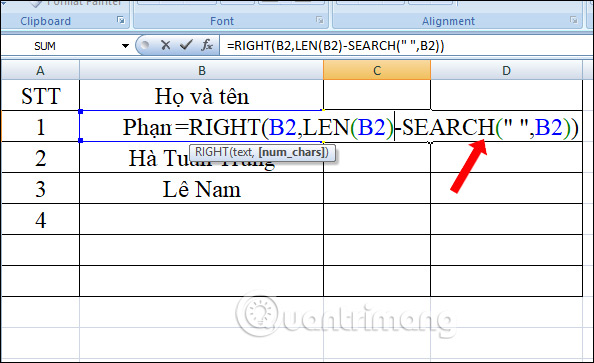
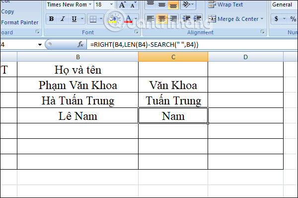
The result is our name as shown below. Scroll down to display the remaining results.

RIGHT function, how to use the right-cut string function in Excel Picture 5

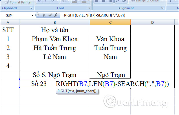
By combining these three functions, we can apply it to output the string of characters after any other character, such as commas, two dots, hyphens, .

RIGHT function, how to use the right-cut string function in Excel Picture 6

Example 4: The RIGHT function of the first n characters in the string

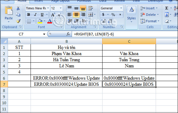
Formula using RIGHT (string, LEN (string) -number of chars to remove) .

In this data table will remove the first 6 characters including the dot from the string. Enter the formula = RIGHT (B2, LEN (B2) -6) and press Enter. The result we get is as shown below.

RIGHT function, how to use the right-cut string function in Excel Picture 7

Example 5: The RIGHT function outputs the character after the last delimiter

With complex strings of multiple delimiters, the content extraction must be separated from the final delimiter. With the data table below, there is a cell that uses only 1 delimiter, but has cells that use 2 delimiters and requires the character after the final delimiter.

Apply the formula to this data table we enter = RIGHT (B6, LEN (B6) -SEARCH ("$", SUBSTITUTE (B6, ":", "$", LEN (B6) -LEN (SUBSTITUTE (B6 , ":", ""))))) and press Enter. Inside:

1. LEN (B6): the total length of the string in cell B6.
2. LEN (SUBSTITUTE (B6, ":", "")): length of character string without a colon.
3. LEN (B6) -LEN (SUBSTITUTE (B6, ":", "")): The total initial length minus the string length without a colon.
4. SUBSTITUTE (B6, ":", "$", LEN (B6) -LEN (SUBSTITUTE (B6, ":", ""))): replace the last separating colon with the new character $, SUBSTITUTE function allows to replace the specified character in the string.
5. SEARCH ("$", SUBSTITUTE (B6, ":", "$", LEN (B6) -LEN (SUBSTITUTE (B6, ":", "")))): determine the location of the final separator , in the colon image, is replaced with the $ sign.
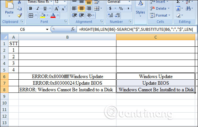
6. RIGHT (B6, LEN (B6) -SEARCH ("$", SUBSTITUTE (B6, ":", "$", LEN (B6) -LEN (SUBSTITUTE (B6, ":", ""))))): Returns the string to the right of the last separator, taking the total string length minus the position of the delimiter.

RIGHT function, how to use the right-cut string function in Excel Picture 8

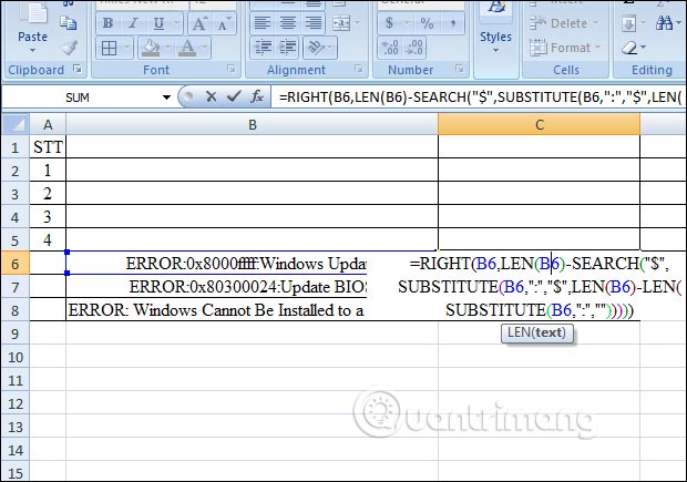
The result is a sequence of characters as shown below.

RIGHT function, how to use the right-cut string function in Excel Picture 9

I wish you all success!