Instructions on how to graph in Excel
Instructions on how to graph in Excel. Excel helps you to process and calculate data effectively, Excel supports you to graph quickly.
Table of Contents
Excel helps you to process and calculate data effectively, Excel supports you to graph quickly.

If you do not know how to graph in Excel, you follow the article below for details on how to graph in Excel.
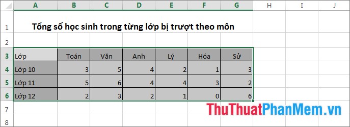
For example, we have the following data table:

HOW TO DRAW AROUND IN EXCEL
Step 1: Select the data area to graph, you need to select the label of the data columns.
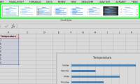
Step 2: Next, select Insert , in the Charts section, select the type of graph you want to draw.

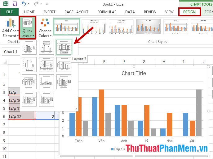
Step 3: At this time, the Excel interface will appear as your selected graph. You can change the layout of the elements on the graph just by selecting the graph, on the Ribbon appears Design tab and Format tab of Chart Tools , select Design -> Quick Layout -> select suitable layout type.
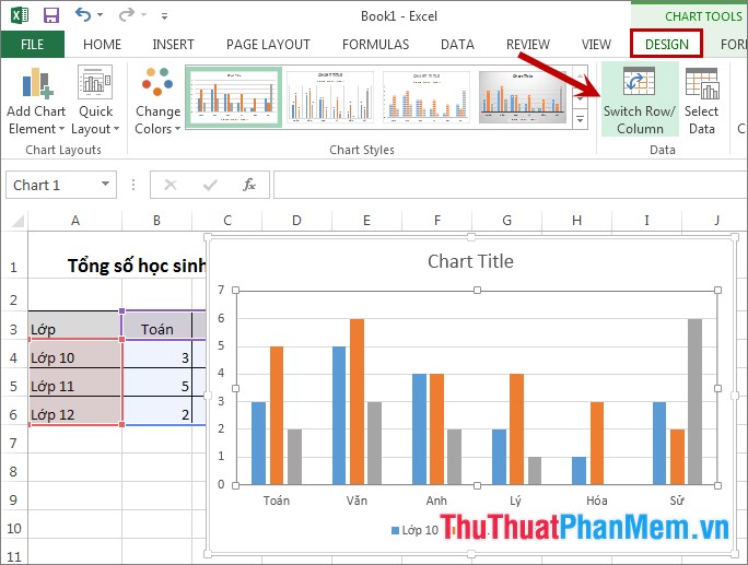
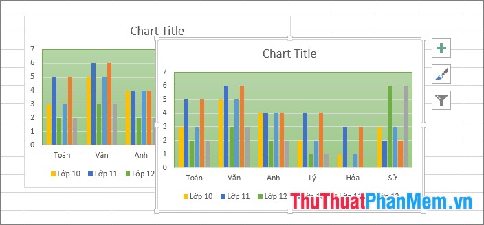
Step 4: You can also change the way of displaying - reversing row and column data in the graph by selecting the graph -> Design -> Switch Row / Column .
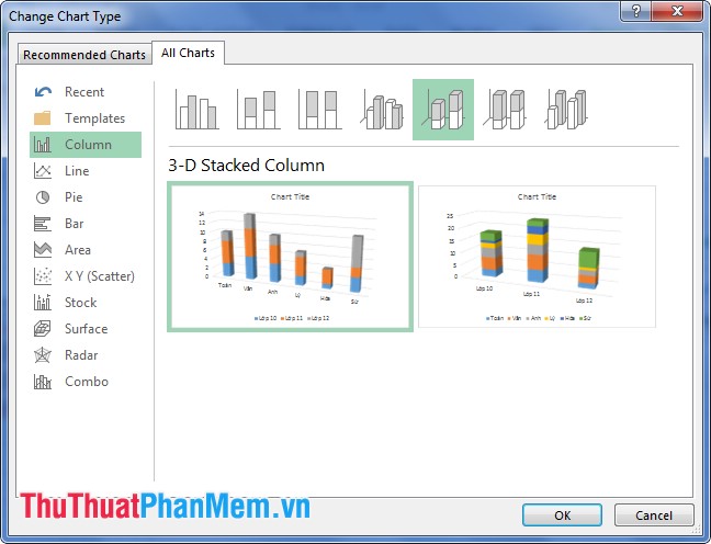
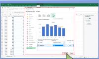
Step 5: If the chart type you choose does not match the data in the data sheet, you can choose another chart type by: selecting graph -> Design -> Change Chart Type .
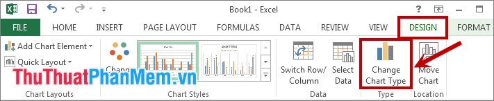
In the Change Chart Type dialog box, select another graph type in the All Charts tab and then click OK to change.
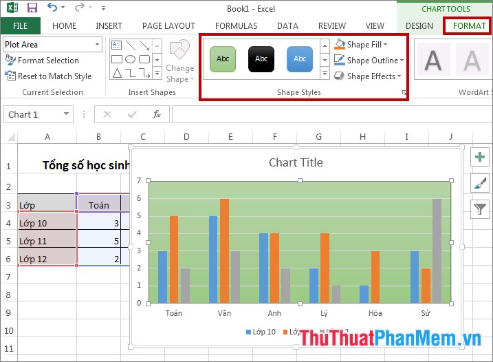
Step 6: Also in the Design tab you can change the colors for the graph in the Chart Styles section .
THE MANUFACTURING WITH GRAPHICS IN EXCEL
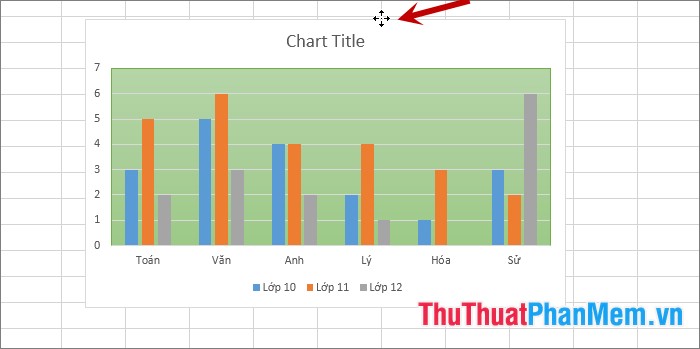
Move graph
Click to select the area of the chart ( Chart Area ), this time the mouse pointer has 4-way arrow icon as shown below. Then hold down the left mouse button and move the graph to where you want to move and release the left mouse button.
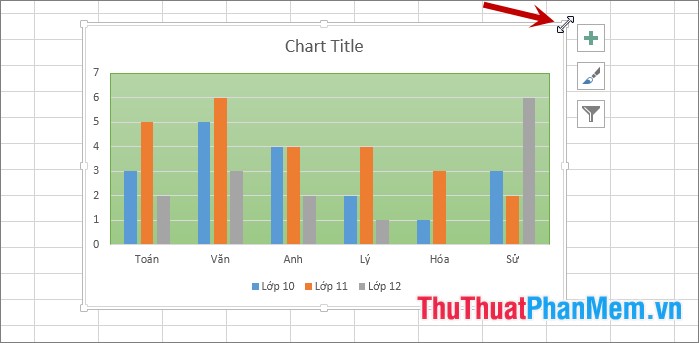
Change the graph size
You click to select the graph area, between the four sides and four corners of the graph area with knobs. You just need to move the mouse cursor to the hold button, then the mouse pointer will turn into a two-way arrow, you hold down the left mouse button and drag outside or inward to zoom in or out the graph.
Copy the graph
You need to select the graph and press Ctrl + C to copy the graph, then select the mouse in any cell you want to copy the graph and press Ctrl + V to paste the graph.
Delete the graph
Select the graph area and press the Delete key on the keyboard to delete the selected graph.
Print the graph
- You can print graphs like other parts of Excel, choose Print Preview before printing to make sure the position of the graph does not cover other Excel content.
- If you only want to print the graph separately, then you select the graph and choose File -> Print to print.

Thus, the article has detailed instructions for you to graph in Excel. Hope the article will help you. Good luck!
Was this article helpful?
Your feedback helps us improve.
Related Articles
 Detailed instructions on how to graph in excel3 minutes read
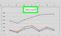 How to Make a Line Graph in Microsoft Excel4 minutes read
 How to Make a Bar Graph in Excel4 minutes read
 How to Add a Second Y Axis to a Graph in Microsoft Excel4 minutes read
 How to Import, Graph, and Label Excel Data in MATLAB5 minutes read
 How to graph functions in Excel4 minutes read
Reader Comments 0
Sign in with email or Google to join the discussion.