How to use VSTACK and HSTACK functions in Excel

Want to know how to stack and append data in Microsoft Excel? Then let's learn how to use the VSTACK and HSTACK functions in Microsoft Excel !

How to use VSTACK and HSTACK functions in Excel Picture 1

Stacking and adding data is extremely important in data transformation and analysis. These tasks allow combining multiple data files, merging columns or rows, and creating a unified view of information. This can be done using two powerful functions, which simplify the process. Those are VSTACK and HSTACK.

By using the VSTACK and HSTACK functions, you can stack and edit data without having to write complex formulas.

What are VSTACK and HSTACK functions in Excel?

VSTACK and HSTACK are two new Excel functions. They are released as text editing functions in 2022 and can be used by Microsoft 365 users. Even basic level Microsoft 365 users can access it. These functions are also among the many features of Excel for the web that can be used to improve work efficiency.

The VSTACK function (short for vertical stack), allows you to append data and stack them vertically. HSTACK is its opposite function, also known as horizontal stack, which allows you to append data horizontally and stack them side by side.

Both functions use the dynamic array environment to add data and stack them into a separate and extensible array. The data here can be a list, an array, data from multiple sheets, a specific header, or the same worksheet.

How to use the VSTACK function in Excel

The VSTACK function syntax is as follows:

=VSTACK(array1,[array2],.)

The array arguments in the function syntax are the arrays you want to concatenate vertically. Let's start with a simple example. Suppose you have two tables. Each board has a corresponding number of letters and numbers. To use VSTACK:

1. In the formula bar, write VSTACK .
2. Select or write the array for the first table in the function and add a comma. The table here is B3:C7.
3. Follow the comma with the array for the second table. Here is E3:F7.

The final syntax is:

=VSTACK(B3:C7,E3:F7)

How to use VSTACK and HSTACK functions in Excel Picture 2

You can also use this function and exclude headers. Here, we have a list of names. If you want to stack them side by side, do the following:

1. Write the VSTACK function .
2. In brackets, write header.
3. Write commas.
4. Write this array for both tables without header.

=VSTACK({"Name","Age"},B3:C8,B11:C16)

How to use VSTACK and HSTACK functions in Excel Picture 3

You can also sort names by combining VSTACK with the SORT function in Excel. You can achieve this by encapsulating the data in the table using the SORT and VSTACK functions.

=VSTACK({"Name","Age"},SORT(VSTACK(B3:C8,B11:C16)))

How to use VSTACK and HSTACK functions in Excel Picture 4

How to use the HSTACK function in Excel

The syntax of HSTACK is:

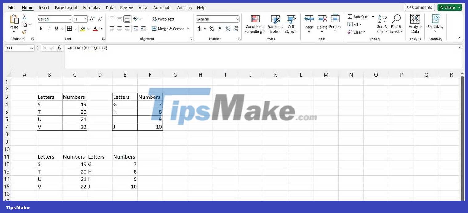
=HSTACK(array1,[array2],.)

The array argument in this function's syntax is the array you want to concatenate horizontally. Let's start with a simple example. Here use letters and numeric data.

1. Write HSTACK in the formula bar.
2. In this function, select or write arrays of tables.

Final syntax:

=HSTACK(B3:C7,E3:F7)

How to use VSTACK and HSTACK functions in Excel Picture 5

Like VSTACK, you can use HSTACK with other functions, like the UNIQUE function in Excel. Let's see how it works. The example here needs a list of unique values ​​from two lists of chocolates. You can include HSTACK in UNIQUE functions.

=UNIQUE(HSTACK(B4:C8, E4:F8))

How to use VSTACK and HSTACK functions in Excel Picture 6

Above is how to use VSTACK and HSTACK in Microsoft Excel . Hope the article is useful to you.

Lesley Montoya

Update 24 July 2023