Instructions for using Index function in Excel

In order to be able to perform data computation in Excel, the table of statistics, the fact that you know the steps to perform or know more tips will help the work to be effective. For example, Excel shortcut keys will help users to shorten the operation, or ways to handle Excel files when problems occur, . Especially to mention the indispensable formula functions when we do work with data table systems in Excel.

Previously, Network Administrator has come to you to read the most basic functions in Excel. These are the most basic functions you'll encounter when working with Excel files, helping us to complete our statistics and calculate our data. And today, we will introduce you to the Index function that is also commonly used in Excel. Index is a function that returns an array, which helps to retrieve values ​​in a certain cell between columns and rows. For a better understanding of how to implement the Index function in Excel, follow our article below.

1. Index Excel functions as Arrays:

The Index function of an array is used for the case if the first argument of the function is an array constant. With this function we have the following formula:

(Array, Row_num, [Column_num])

Inside:

1. Array : a range of cells or a number of certain arrays required.
2. Row_num : select the row in the array from which to return a value.
3. Column_num : select the column in the array from which to return a value.

Readers should note that there must be at least one Row_num and Column_num argument.

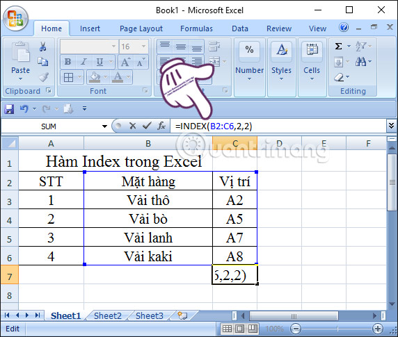
Table Excel 1 : We have a list of fabrics, find the type of fabric that knows the fabric in row 2 column 2.

Step 1:

In cell C7, you will enter the above formula according to the syntax below, and then we press Enter to execute the Index function

C7: = INDEX (B2: C6,2,2)

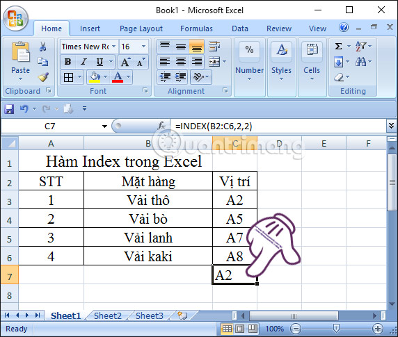
Step 2:

Soon we will return the position value A2 corresponding to the Rough row type.

2. Reference Excel function form:

The Index function of the reference form returns the cell's reference to the intersection of a row and a specific column. We have the Index formula of reference form as follows:

INDEX (Reference, Row_num, [Column_num], [Area_num])

Inside:

1. Reference : mandatory reference area.
2. Row_num : the row number from which returns a reference, required.
3. Column_num : column number from which to return a reference, optional.
4. Area_num : the number of cell range that will return the value in the Reference. If Area_num is omitted, INDEX uses area 1, optional.

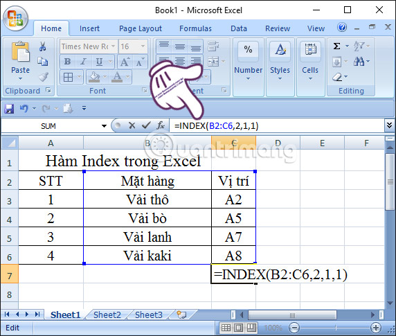
Step 1:

Also with the Excel data table above, we enter the formula as below. Then press Enter.

Click in cell C7: = INDEX (B2: C6,2,1,1)

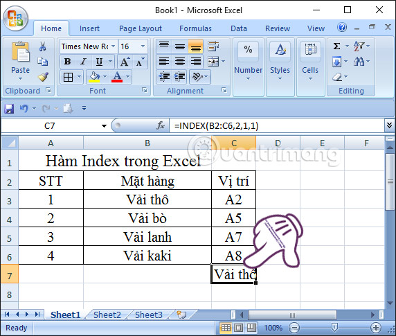
Step 2:

The returned result will be the name of the type of Crude item in line B2.

So, we showed you how to use the INDEX function as an array and reference form. Index function can refer to any cell in Excel, and the implementation is not too difficult. You can use this function and combine with other functions in Excel to make more efficient use of spreadsheet data.

Refer to the following articles:

1. Summary of expensive shortcuts in Microsoft Excel

1. You want to print text, data in Microsoft Excel. Not as simple as Word or PDF! Read the following article!

1. 10 ways to recover corrupted Excel files

I wish you all success!