Basic functions in Excel, calculation formulas and illustrative examples

Excel is an indispensable tool in all office work, from data management to calculation and analysis. If you are not familiar with basic functions in Excel , this article of Free Download will guide you from A to Z.

Basic functions in Excel, calculation formulas and illustrative examples Picture 1

Basic Excel functions, formulas and how to use them 
 

Note: In the instructions below, Free Download will show you how to calculate basic functions in Excel 2016, readers can do it in other versions of MS Excel.
 

1. SUM function: Calculates the total value of cells

To sum the values ​​in selected cells, you use the SUM function with the syntax: =SUM(Number1, Number2.) . Where: Number1, Number2, . are the numbers, cells, or data ranges to sum. You can add as many arguments as you like, as long as you do not exceed Excel's limits.

There are 3 common ways to declare the SUM function:

- Method 1: Calculate the total value in a range of cells

For example, if you have values ​​from cells A1 to A5, and want to sum from A1 to A5, the formula would be: =SUM(A1:A5)

Result: The function =SUM(A1:A5) will return 150.

Basic functions in Excel, calculation formulas and illustrative examples Picture 2 Basic functions in Excel: SUM function

- Method 2: Calculate the sum of specific values

For example: If the values ​​from cells A1 to A5 are: 10, 20, 30, 40, 50, you enter these values ​​into the function with the syntax: =SUM(10;20;30;40;50)

Result: The function returns 150.

Basic functions in Excel, calculation formulas and illustrative examples Picture 3

- Method 3: Calculate the sum of non-adjacent areas

You can add multiple non-contiguous regions by separating them with semicolons:

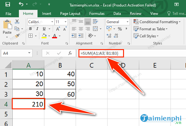
For example: If you want to calculate the sum of the range A1 to A3 and the range B1 to B3, the syntax would be: =SUM(A1:A3; B1:B3)

Basic functions in Excel, calculation formulas and illustrative examples Picture 4
 

2. IF condition function

If you want to filter values ​​in an Excel spreadsheet, you need to use the IF function with the syntax:  =IF(logical_test; value_if_true; value_if_false)

In there:

- logical_test: Is the condition to be checked.

- value_if_true: The value returned if the condition is true.

- value_if_false: The value returned if the condition is false.

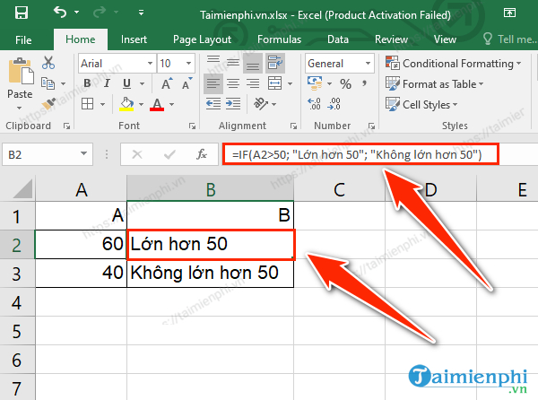
For example, if you want to check if the value in cell A2 is greater than 50, the syntax would be =IF(A2>50; "Greater than 50"; "Not greater than 50")

- If the value in A2 is greater than 50, the function returns "Greater than 50".

- Otherwise, the function returns "Not greater than 50".

Similarly, If you want to check if the value in cell A3 is greater than 50, the syntax would be =IF(A3>50; "Greater than 50"; "Not greater than 50")

Basic functions in Excel, calculation formulas and illustrative examples Picture 5 Basic functions in Excel: IF function
 

3. Function to get the left character (LEFT)

The LEFT function in Excel is used to get characters from the left side of a string (can take multiple characters), syntax: =LEFT(text; [num_chars]).

In there:

- text: Text string to get characters from.

- num_chars: (Optional) Number of characters to get from the left side of the string.

If num_chars is omitted, the function defaults to 1 character.

For example, if you want to get the first character from the names in column A, the formula would be: =LEFT(A1; 1)
 

Basic functions in Excel, calculation formulas and illustrative examples Picture 6
 

4. Get the right character (RIGHT)

Similar to the LEFT function, the RIGHT function helps you get the right value of a string, you can get more than 1 character in that string. Syntax: =RIGHT(text; num_chars)

In there:

- text: Text string to get characters from.

- num_chars: (Optional) Number of characters to get from the right side of the string.

If num_chars is omitted, the function defaults to 1 character.

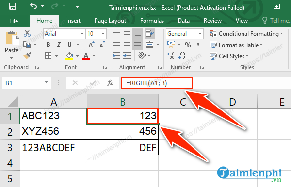
For example, let's say you have a list of product codes in column A, and you want to get the last 3 characters of each code, the syntax would be: =RIGHT(A1; 3) 

Basic functions in Excel, calculation formulas and illustrative examples Picture 7 Basic functions in Excel: RIGHT function
 

5. MIN function: Function to find the smallest value

The MIN function finds the smallest value in selected cells or ranges.
Syntax: =MIN(number1; [number2], .)

Suppose you have a list of numbers in column A from cells A1 to A5: 3; 45; 12; 67; 34. To find the smallest value, you enter the syntax: =MIN(3; 45; 12; 67; 34).

Basic functions in Excel, calculation formulas and illustrative examples Picture 8
 

6. MAX function: Function to find the largest value

The MAX function finds the largest value in selected cells or ranges.  Syntax: =MAX (number1; [number2], .)

For example, suppose you have a list of numbers in column A from cells A1 to A5: 3; 45; 12; 67; 34. To find the largest value, you enter the syntax: =MAX(3; 45; 12; 67; 34).

Basic functions in Excel, calculation formulas and illustrative examples Picture 9
 

7. AVERAGE function

The AVERAGE function is one of the basic functions in Excel that allows you to calculate the average value of selected cells or ranges. Using the AVERAGE function, you will perform simpler calculations.

Syntax: =AVERAGE(number1; [number2], .)

For example, suppose you have a list of numbers in column A from cell A1 to A5 respectively: 10;20;30;40;50. The formula to calculate the average from column A1 to A5 is: =AVERAGE(A1:A5) or =AVERAGE(10;20;30;40;50).

Basic functions in Excel, calculation formulas and illustrative examples Picture 10
 

8. TRIM function to trim spaces

The TRIM function is a basic Excel function that helps remove spaces between characters in a string and leaves only one space (equal to 1 space between words). With many cells containing strings with many spaces, the TRIM function is really useful.

Syntax: =TRIM(text)

In which: Text is the text containing the space to be removed is 1

Example :  The text string in cell A1 is: Hello December, to remove extra spaces in the text string, enter the following syntax: =TRIM(A1).
 

9. CONCATENATE string concatenation function

The CONCATENATE function is a function that concatenates character strings in Excel spreadsheets. Using the CONCATENATE function , you will not have to manually concatenate word strings together.

Syntax: =CONCATENATE (text 1; text 2; …)

In which: Text 1: is the first string (this is a required string)

Text 2 …: optional, maximum 255 strings, and strings must be separated by commas

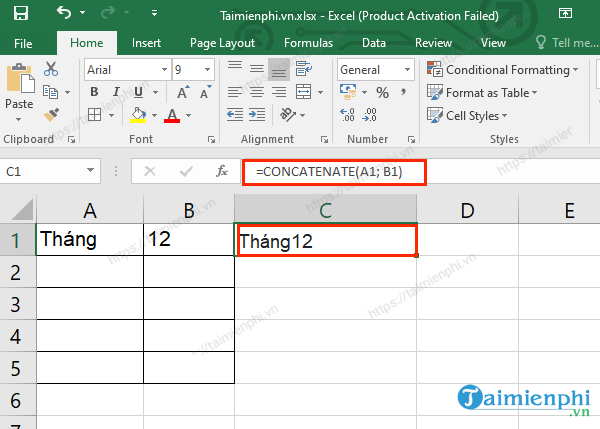
Let's say cell A1 has "Month", and cell B1 has "12". To concatenate two text strings from two cells, you enter the formula: =CONCATENATE(A1; B1)

Basic functions in Excel, calculation formulas and illustrative examples Picture 11 Basic functions in Excel: CONCATENATE function 
 

10. COUNT function: Function to count numeric data 

The COUNT function is a basic excel function that counts data. Using the Count function , you will count the number of numeric data in an excel spreadsheet.  Syntax: =COUNT(value1; [value2]; .)

For example, to count the number of numeric values ​​in the range from columns A to E in the table below, you follow the formula: =COUNT(A1:E1).

Basic functions in Excel, calculation formulas and illustrative examples Picture 12
 

11. COUNTA function: Function to count cells containing data

The COUNTA function counts cells that contain data.

Syntax: =COUNTA(value1; [value2]; .)

For example: We have data in the range in the data table from column A to column E. To count the number of cells with data in the range, you enter the formula: =COUNTA(A1;B1;C1;D1;E1).

Basic functions in Excel, calculation formulas and illustrative examples Picture 13 Basic functions in Excel: COUNTA function
 

12. Function to count the length of a character string

The LEN function is a basic Excel function that helps you count the length of a string of characters. The LEN function will return the value that is the length of the string of characters, including white space characters.  Syntax: =LEN (text)

In which: Text: is a string of characters

For example: If you want to count the number of characters in cell B1. You use the syntax =LEN(B5). The result will be as shown. To count the next cells, you just need to hold the mouse at I5 and drag down.
 

13. Function to display current time on the system NOW

NOW function returns the current date on the system
Syntax: =NOW ()
 

14. SUMIF function: Function to sum cells with conditions

The SUMIF function is a basic function in Excel that allows you to calculate the sum of cells or ranges whose values ​​satisfy the given conditions.  Syntax: =SUMIF(range; criteria; [sum_range]) .

Cells containing Criteria conditions: Sum_range conditions: Cells to calculate the sum
Example: To calculate the total score for students with scores above 8 in the list below, enter the formula: =SUMIF(B2:B6; ">8")

Basic functions in Excel, calculation formulas and illustrative examples Picture 14 Basic functions in Excel: SUMIF function
 

15. COUNTIF function: Function to count data with conditions

The COUNTIF function counts cells that satisfy a condition.  Syntax: =COUNTIF(range; criteria)

For example: To count the number of students with scores above 8, the formula is: =COUNTIF(B2:B6; ">8").

Basic functions in Excel, calculation formulas and illustrative examples Picture 15
 

16. COUNTBLANK function: Function to count empty data

The COUNTBLANK function in Excel is used to count the number of cells in a range that do not contain any data, i.e. blank cells. This is a useful function when you want to know how many blank cells there are in a range of cells you are working with.

Syntax: =COUNTBLANK(range)

Example: Count the number of blank cells in a data range, formula: =COUNTBLANK(B2:B6)

Basic functions in Excel, calculation formulas and illustrative examples Picture 16
 

When working with Excel, you need to understand the basic functions in Excel to be able to use Excel most effectively and quickly. Excel functions commonly used in basic offices such as Sum, Min, Max . support a lot in your study and work.

Above are some basic functions in Excel. Excel is a very convenient and popular office software that supports calculations. You can refer to the most common Excel shortcuts to operate the software faster.

In addition to basic functions in Excel, readers should also refer to advanced functions such as VLOOKUP, CHOOSE . to improve their knowledge. Advanced functions in Excel are applied to make calculations on Excel spreadsheets faster.

David Pac

Update 09 December 2024