Common Excel functions you need to know about accounting

Common Excel functions you need to know about accounting Picture 1

In addition to professional accounting software such as Misa, Fast, Mcom ., Excel is a popular software used in the work of accountants. Mastering the common Excel functions helps accountants save time and effort compared to conventional manual calculations. Today, Software Tips will list and guide readers on how to use some functions commonly used in accounting.

Addition and Subtraction Division

Summation

Syntax = SUM (number1, [number2], .)

Inside:

1. SUM : is a function used to calculate totals.
2. Number1: is the first argument.
3. Number2, .: is the 2nd argument onwards (may or may not).

Arguments can be a data range, a number, a single cell reference, and are separated by commas (,).

Or you can use the plus sign (+) to perform addition.

Common Excel functions you need to know about accounting Picture 2

Subtraction

Syntax: = number1 - number2

Inside:

1. Minus sign (-):  is a calculation operator used to perform subtraction.
2. Number1: the number to be deducted.
3. Number2: the minus number.

Number can be a number or the position of a cell containing data.

For example: You type: = 5-2 in cells => the result is 3.

Multiplication

Syntax: = PRODUCT (number1, [number2], .)

Inside:

1. PRODUCT : is a function used to multiply factors .
2. Number1: is the 1st factor.
3. Number2, .: is the second factor onwards (may or may not).

Numbers can be a data range, a number, a single cell reference, and are separated by commas (,).

Or you can use the asterisk (*) to perform multiplication.

For example: You type the formula: = PRODUCT (2,6,9) in a cell => the result is 108.

Division

Syntax: = number1 / number2

Inside:

1. The forward slash (/): is the calculation operator used to perform the division operation.
2. Number1: is the divided number.
3. Number2: is the divisor.

Number can be a number or the position of a cell containing data.

For example: You type in a cell: = 10/3 => the result is 3,33333 .

AVERAGE function

Syntax: = AVERAGE ( number1, [number2], . )

Inside:

1. AVERAGE: is the function name used to calculate the average of the arguments.
2. Number1: is the first argument.
3. Number2, .: is the 2nd argument onwards (may or may not).

Arguments can be a data range, a number, a single cell reference, and are separated by commas (,).

For example: = AVERAGE (1,2,3) => returns 2.

SUBTOTAL function

Syntax: = SUBTOTAL (function_num, ref1, [ref2], .)

Inside:

1. SUBTOTAL : is the name of the function used to calculate the displayed lines. The lines hidden by the filter will be ignored.
2. Function_num: values ​​1-11 or 101-111 specify the function to use for subtotals. 1-11 include hidden rows manually, while 101-111 excludes them; Filtered cells will always be excluded.
3. Ref1 : is the first named range or reference to which you want to subtotal.
4. Ref2 , .: optional values. The range or series is named from 2 to 254 that you want to subtotal for it.

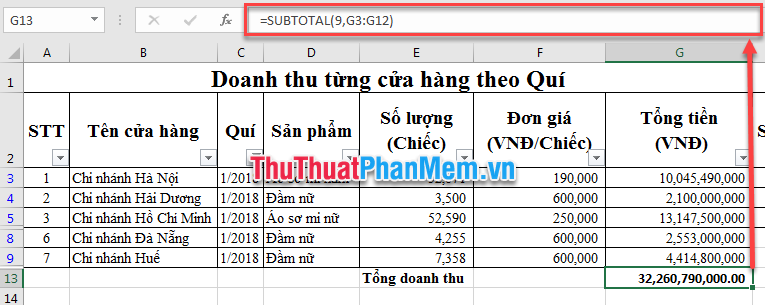
For example, if you want to sum the filtered rows with the Filter tool , in the totals box, use the formula: = SUBTOTAL (9, G3: G12) . Where 9 : is the total requirement, G3: G12 is the data container for which the formula is applied. When we use the filtering tool to request information, the total cell will only add the rows that are filtered.

Total filtered revenue by Hanoi Branch:

Common Excel functions you need to know about accounting Picture 3

Total filtered revenue by Q1 / 2018:

Common Excel functions you need to know about accounting Picture 4

Search function (VLOOKUP and HLOOK UP)

VLOOKUP

Function syntax: = VLOOKUP (lookup_value, table_array, col_index_num, [range_lookup])

Inside:

1. VLOOKUP: is the name of the function used to search data vertical (vertical).
2. lookup_value: is the value to search
3. table_array: is the reference table.
4. col_index_num: number of columns in the reference table that need to return the value.
5. [range_lookup]: optional argument. Returns an approximate or exact match - only two values ​​are declared as 1 / TRUE (approximate), or 0 / FALSE (exact).

For example, if you have the unit price table to fill out, you use the VLOOKUP function according to the following formula:

Common Excel functions you need to know about accounting Picture 5

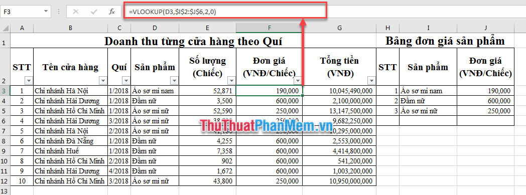
Note:

1. The first column must contain data to reference.
2. The reference region must always be absolute. (Unless you have other requirements).
3. If VLOOKUP returns the # N / A error value if the value to look for is not in the reference table. You should check the reference table and supplement the information.

HLOOKUP function

Function syntax: = HLOOKUP (lookup_value, table_array, row_index_num, [range_lookup])

Inside:

1. HLOOKUP: is the name of the function used to search data horizontally.
2. lookup_value: is the value to search
3. table_array: is the reference table.
4. row_index_num: number of columns in the reference table that need to return the value.
5. [range_lookup]: optional argument. Returns an approximate or exact match - only two values ​​are declared as 1 / TRUE (approximate), or 0 / FALSE (exact).

The way to use HLOOKUP is similar to VLOOKUP, except for HLOOKUP, which searches for data by line.

IF function

Function structure: = IF (Logical_test, [value_if_true], [value_if_false])

Inside:

1. IF: is the name of the conditional function will return value 1, if condition is true, and value 2 if condition is false.
2. Logical_test: is the reference condition.
3. [value_if_true]: optional argument. Is the return value if the Logical_test condition is true. If the user does not enter value_if_true , Excel will return TRUE if the condition is true.
4. [value_if_false]: optional argument. Is the return value if the Logical_test condition is false. If the user does not enter value_if_false value , Excel will return FALSE value if the condition is false.

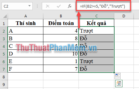
For example, you have the following scoreboard to classify:

1. Candidates greater than or equal to 5 points => Do.
2. Candidates under 5 points => failed.
   We use the formula for cell C2 as; = IF (B2> = 5, "Do", "Slide").

Common Excel functions you need to know about accounting Picture 6

SUMIF and SUMFIS functions

SUMIF function structure: = SUMIF (range, criteria, sum_range)

Inside:

1. SUMIF: is the function name used to calculate the total under a required condition.
2. Range: is the reference area containing condition data.
3. Criteria: a condition that needs to be satisfied.
4. sum_range: is the area to sum.

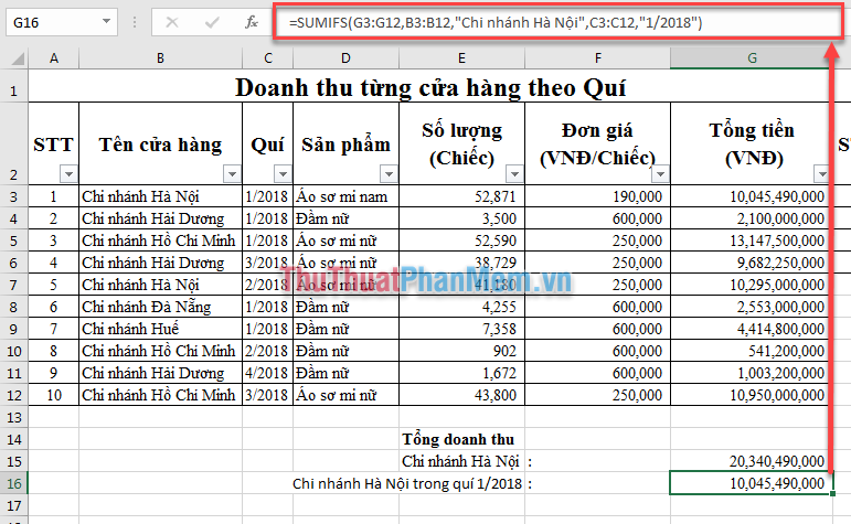
For example: You have the sales table as shown below, and need to calculate the total sales of Hanoi branch, You type the formula into a cell in Excel spreadsheet = SUMIF (B3: B12, "Hanoi Branch", G3 : G12).

Common Excel functions you need to know about accounting Picture 7

SUMIFS function structure: = SUMIFS sum_range, criteria_range1, criteria1, [criteria_range2, criteria2], .)

Inside:

1. SUMIFS: is the function name used to calculate the sum of many conditions.
2. sum_range: is the area to sum.
3. criteria_range1,2,3 .: is the reference area containing the conditional data 1,2,3 .
4. Criteria1,2,3 .: is a condition that requires 1,2,3 .

With the above sales example, we need to calculate the sales of Hanoi Branch in the first quarter of 2018, we use the formula: = SUMIFS (G3: G12, B3: B12, "Hanoi Branch", C3: C12 , "1/2018").

Common Excel functions you need to know about accounting Picture 8

AND AND OR functions

Function structure: = AND (Logical1; [Logical2]; [Logical3]; .)

Inside:

1. AND: means the function name means AND, and returns the TRUE result when all arguments are true.
2. Logical1,2,3 .: Arguments are constants, logical expressions.

Function structure: = OR (Logical1; [Logical2]; [Logical3]; .)

Inside:

1. OR: is the name of the function that means OR, and returns the FALSE result when all arguments are false.
2. Logical1,2,3 .: Arguments are constants, logical expressions.

Examples distinguish AND and OR:

AND (TRUE, FALSE) = FALSE

OR (TRUE, FALSE) = TRUE.

MIN and MAX functions

Function structure: = MIN ( number 1, number 2, .)

Inside:

1. MIN: is the function name used to return the smallest value in the series.
2. number 1,2 .: is the number sequence to find the minimum value.

Function structure: = MAX ( number 1, number 2, .)

Inside:

1. MAX: is the name of the function used to return the maximum value in the series.
2. number 1,2 .: is the number sequence to find the minimum value.

For example: MIN (10,5,16) = 5 and MAX (10,5,16) = 16.

LEFT, RIGHT, MID functions

The LEFT, RIGHT, MID functions allow the user to retrieve some characters from the string.

Syntax:

= LEFT (text, [num_chars]) .
= RIGHT (text, [num_chars]) .
= MID (text, start_num, num_chars).

Inside:

1. LEFT: is the name of the function to extract characters from left to right of the text string.
2. RIGHT: is the name of the function to extract characters from right to left of the text string.
3. MID: is the name of the function that you want to extract characters from start_num that you specify from left to right.
4. Text : The text string containing the characters you want to extract.
5. Start_num: the number of the character that the MID function starts to retrieve.
6. Num_chars : Specify the number of characters you want LEFT / RIGHT to extract. Num_chars must be greater or equal to zero. If num_chars is greater than the length of the text, LEFT / RIGHT returns the entire text. If num_chars is omitted, it is defaulted to 1.

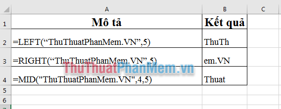
For example, you have the string "TipsMake.VN", you take 5 characters on the left, 5 characters on the right, and 5 characters from the 4th character;

= LEFT ("TipsMake.VN", 5) => the result is: ThuTh;
= RIGHT ("TipsMake.VN", 5) => the result is: em.VN;
= MID ("TipsMake.VN", 4,5) => The result is: Thuat .

Common Excel functions you need to know about accounting Picture 9

TEXT FUNCTION

Syntax: = TEXT (number, format)

Inside:

1. TEXT : is the name of the function used to change the display of numbers.
2. Number : is the number to be formatted.
3. Format : the format code you want to apply.

The TEXT function is used to convert numbers to regular letters, or to format numbers as dates, percentages, currencies, etc.

Here are some common format codes that Software Tips introduces to you:

Description

Some sample code format

"# .000" :

Rounds the number and represents the 3rd fraction (automatically adds the zero to the missing position).

Example: TEXT (2.7, "#. 000") = 2,700

"#. ##"

Rounds a number and shows it to the 2nd fraction and does not show 0.

For example: TEXT (2,7856, "#. ##") = 2.79

"?????. ??"

Add leading and rounding spaces, representing the 2nd fraction.

For example: TEXT (2.7, "?????. ??")) = ˽˽˽˽2.7

"#, ###. 00"

Use thousands and 2 decimal separators

Example: TEXT (1234567.99, "###, ###, ###. 00") = 1,234,567.99

"$ #, ###. 00"

Add currency format with thousand separator and two decimal places.

Example: = TEXT (1234567.99, "$ #, ###. 00") = $ 1,234,567.99

"% .00"

Add currency format with two decimal places.

For example: = TEXT (2.7, "% .00") =% 270.00

"MM / DD / YY"

Format month / day / year.

For example: TEXT (TODAY (), "MM / DD / YY") = March 7, 19

"H: MM AM / PM"

Time format: minute am / pm.

For example: TEXT (NOW (), "H: MM AM / PM") = 0:41 PM.

Above Software Tips guide you some of the functions commonly used in accounting. Hope this article will be helpful for you. Good luck!