How to Sort Excel Columns Alphabetically

Sort alphabetically

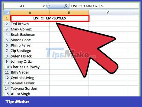
Format the headline. The header line is the first line in the spreadsheet, containing the name of the column. Sometimes Excel will sort this entire line because it thinks it's part of the data, especially if your spreadsheet is all text. Here are a few ways to prevent this:

Format the headline differently. For example, you can highlight or change the color of text.

You need to make sure there are no blank cells in the subject line.

If Excel still sorts, select the headline and, using the top ribbon menu, click Home → Editing → Sort & Filter → Custom Sort sort) → My data has headers.

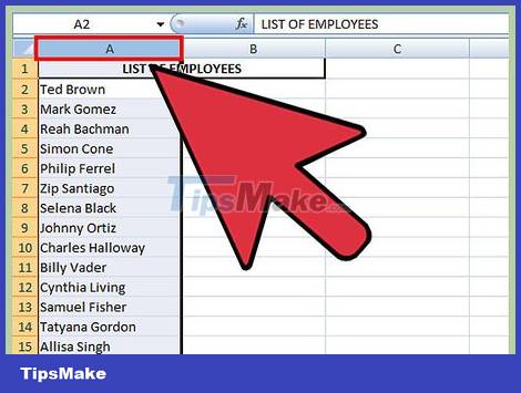
Select the column to sort. You can click a column's title box or the letter above it (A, B, C, D, etc.).

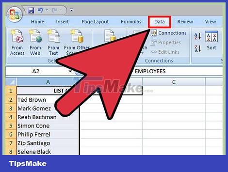
Open the Data tab. Click the Data tab in the top menu of the screen to see data options in the ribbon menu above the spreadsheet.

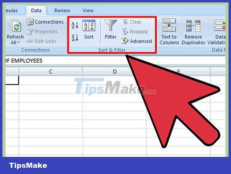
Find the Sort and Filter section. The ribbon menu is divided by region with names below. Look for the area labeled Sort & Filter.

If you can't find it in the Data menu, try going back to the Home tab and looking for the Sort & Filter button in the Editing section.

Click the A → Z button. If you want to sort the spreadsheet alphabetically, just click the A → Z icon in the Sort and Filter section. The selected column will be rearranged in alphabetical order. On most versions of Excel, this button is usually located in the upper left corner of the Sort and Filter section.

If you want to sort in reverse alphabetical order, click Z → A.

Sort by last name (applies to English name structure)

This method applies when the spreadsheet includes first and last names in one cell. If you have a list of full names (first name first, last name later) in a separate column, sorting will be by first name only. With the following instructions, you will be able to divide the full name into two columns and then sort by the last name column.

Insert a new blank column. Place this column immediately to the right of the full name column.

Enter the formula for the name. Enter this formula in the top cell of the new column: =LEFT(A1,FIND(" ",A1)) and make sure there are spaces within the quotes. This formula will look in the full name column and copy any data before the space.

If necessary, you can replace A with the letter of the column name containing the list of first and last names.

Replace the number 1 with the line number you are entering.

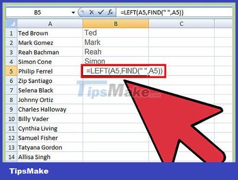
Copy this formula for the entire column. Click the new column header, copy and paste the formula you just entered. You will see all names automatically appear in this column.

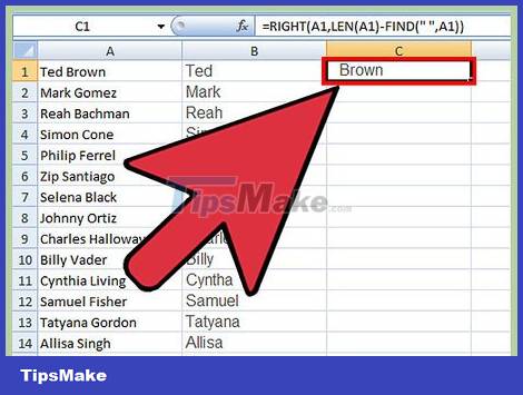
Create a last name column. Create a new column to the right of the name column. Copy and paste this formula to populate the column with last names:

=RIGHT(A1,LEN(A1)-FIND(" ",A1))

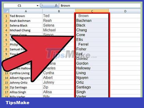
Sort by last name column. You can now sort the last name column alphabetically, as described above.

Jessica Tanner

Update 10 November 2023