Row: How to Copy Formulas in Excel

This updated guide examines Row: How to Copy Formulas in Excel and organizes the essential facts, background, and practical takeaways in clear American English.

Method 1

Copying a Formula into Multiple Cells by Dragging

1. Enter the formula into one cell. As with any formula, start with an = sign, then use whichever functions or arithmetic you'd like. We'll use a simple example spreadsheet, and add column A and column B together: Example Spreadsheet Column AColumn BColumn Crow 1

   9

   =A1+B1

   row 2

   20

   8

   row 3

   30

   7

   row 4

   40

   6

2. Press enter to calculate the formula. Once you hitenteron your keyboard, the formula will be entered and calculated. Only the result (19) will be displayed, but the spreadsheet will still have the formula stored. Example Spreadsheet Column AColumn BColumn Crow 1

   10

   9

   19

   row 2

   20

   8

   row 3

   30

   7

   row 4

   40

   6

3. Click on the lower right corner of the cell to be propagated. Move your cursor to the lower right corner of the cell you just edited. The cursor will become a bold + sign.^{[1]XResearch source}
4. Hold and drag along the column or row you're copying to. Keep your mouse button held down, and drag your cursor down the column, or across the row to be edited (highlight). The formula you entered will automatically be entered into the cells you've highlighted. Relative cell references will automatically update to refer to the cell in the same relative position. Here's our example spreadsheet, showing the formulas used and the results displayed: Example Spreadsheet Column AColumn BColumn Crow 1

   10

   9

   =A1+B1

   row 2

   20

   8

   =A2+B2

   row 3

   30

   7

   =A3+B3

   row 4

   40

   6

   =A4+B4

   Example Spreadsheet Column AColumn BColumn Crow 1

   10

   9

   19

   row 2

   20

   8

   28

   row 3

   30

   7

   37

   row 4

   40

   6

   46

5. Double click the plus sign to fill the entire column. Instead of click-and-dragging, move your mouse to the lower right corner, and double click when the cursor turns into a + sign. This will automatically copy the formula to the entire column.^{[2]XResearch source}
   • Excel will stop filling out the column if it sees an empty cell. If the reference data contains a gap, you will have to repeat this step to fill out the column below the gap.

Method 2

Copying a Formula into Multiple Cells by Pasting

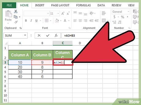1. Enter the formula into one cell. As with any formula, start with an = sign, then use whichever functions or arithmetic you'd like. We'll use a simple example spreadsheet, and add column A and column B together: Example Spreadsheet Column AColumn BColumn Crow 1

   10

   9

   =A1+B1

   row 2

   20

   8

   row 3

   30

   7

   row 4

   40

   6

2. Press enter to calculate the formula. Once you hitenteron your keyboard, the formula will be entered and calculated. Only the result (19) will be displayed, but the spreadsheet will still have the formula stored. Example Spreadsheet Column AColumn BColumn Crow 1

   10

   9

   19

   row 2

   20

   8

   row 3

   30

   7

   row 4

   40

   6

3. Click on the cell to be propagated and copy it (CTRL+C).
4. Select the cells you want to copy the formula to. Click on one and drag up or down using your mouse or the arrow keys. Unlike with the corner drag method, the cells you are copying the formula to do not need to be adjacent to the cell you are copying from.
5. Paste (CTRL+V).

Method 3

Copying a Formula Exactly

1. Use this method to quickly copy a formula without changing the cell references. Sometimes, you have a large spreadsheet full of formulas, and you want to copy them exactly . Changing everything to absolute cell references (as described in the section on cell references) would be tedious, especially if you just want to change them back again afterward. Use this method to quickly move formulas with relative cell references elsewhere without changing the references.^{[3]XResearch source}Here's our example spreadsheet, which needs to have column C duplicated to column D: Example Spreadsheet Column AColumn BColumn CColumn Drow 1

   944

   Frogs

   =A1/2

   row 2

   636

   Toads

   =A2/2

   row 3

   712

   Newts

   =A3/2

   row 4

   690

   Snakes

   =A4/2

   • If you're just trying to copy the formula in a single cell, skip to the last step ("Try alternate methods") in this section.
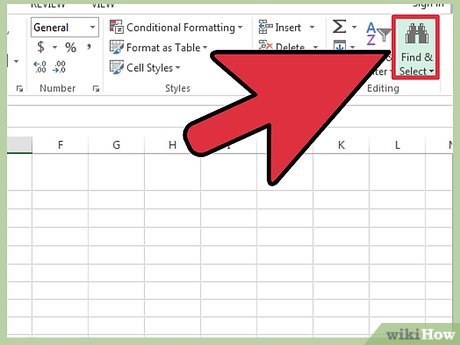2. Open the Find window. On most versions of Excel, you can find this by clicking theHometab at the top of the Excel window, then clickingFind & Selectin the "Editing" portion of the tab.^{[4]XResearch source}You can also use the keyboard shortcut, CTRL F.
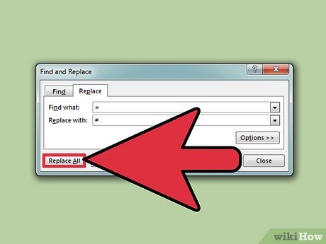3. Find and replace "=" with another character. Enter "=", click "Find All," then enter another character into the "Replace with" box. This will automatically turn all formulas (which always begin with =) into text strings beginning with some other character. Always use a character that you have not used in your spreadsheet. For example, replace it with # or &, or a longer string of characters, such as ##&. Example Spreadsheet Column AColumn BColumn CColumn Drow 1

   944

   Frogs

   ##&A1/2

   row 2

   636

   Toads

   ##&A2/2

   row 3

   712

   Newts

   ##&A3/2

   row 4

   690

   Snakes

   ##&A4/2

   • Do not use the characters * or?, since these will make later steps more difficult.
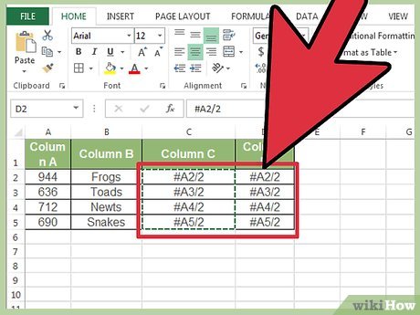4. Copy and paste the cells. You may now select any cells you wish to copy, then paste them into another location. Since they are no longer interpreted as formulas, they will be copied exactly. Example Spreadsheet Column AColumn BColumn CColumn Drow 1

   944

   Frogs

   ##&A1/2

   ##&A1/2

   row 2

   636

   Toads

   ##&A2/2

   ##&A2/2

   row 3

   712

   Newts

   ##&A3/2

   ##&A3/2

   row 4

   690

   Snakes

   ##&A4/2

   ##&A4/2

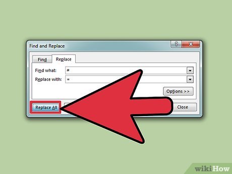5. Use Find & Replace again to reverse the change. Now that you have the formulas where you want them, use the "Find all" and "Replace with" options to reverse your change. In our example, we'll look for the character string "##&" and replace it with "=" again, so those cells become formulas once again. You can now continue editing your spreadsheet as usual: Example Spreadsheet Column AColumn BColumn CColumn Drow 1

   944

   Frogs

   =A1/2

   =A1/2

   row 2

   636

   Toads

   =A2/2

   =A2/2

   row 3

   712

   Newts

   =A3/2

   =A3/2

   row 4

   690

   Snakes

   =A4/2

   =A4/2

6. Try alternate methods. If the method described above does not work for any reason, or if you are worried about accidentally changing other cell contents with the "Replace all" option, there are a couple other methods you can try:
   • To copy a single cell's formula without changing references, select the cell, then copy the formula shown in the formula bar near the top of the window (not in the cell itself). Pressescto close the formula bar, then paste the formula wherever you need it.^{[5]XResearch source}
   • PressCtrl`(usually on the same key as ~) to put the spreadsheet in formula view mode. Copy the formulas and paste them into a text editor such as Notepad or TextEdit. Copy them again, then paste them back into the spreadsheet at the desired location.<sup>[6]XResearch source</sup>PressCtrl`again to switch back to regular viewing mode.

Method 4

Using Relative and Absolute Cell References

1. Use a relative cell reference in a formula. In an Excel formula, a "cell reference" is the address a cell. You can type these in manually, or click on the cell you wish to use while you are entering a formula. For example, the following spreadsheet has a formula that references cell A2: Relative References Column AColumn BColumn Crow 2

   50

   7

   =A2*2

   row 3

   100

   row 4

   200

   row 5

   400

2. Understand why they're called relative references. In an Excel formula, a relative reference uses the relative position of a cell address. For example: cell C2 has the formula '=A2', which is a relative reference to the value two cells to the left. If you copy the formula into cell C4, then it will still refer to two cells to the left, now showing '=A4'. Relative References Column AColumn BColumn Crow 2

   50

   7

   =A2*2

   row 3

   100

   row 4

   200

   =A4*2

   row 5

   400

   • This works for cells outside of the same row and column as well. If you copied the same formula from cell C1 into cell D6 (not shown), Excel would change the reference "A2" to a cell one row to the right (C?D) and 5 rows below (2?7), or "B7".
3. Use an absolute reference instead. Let's say you don't want Excel to automatically change your formula. Instead of using a relative cell reference, you can make it absolute by adding a $ symbol in front of the column or row that you want to keep the same, no matter where you copy the formula too.^{[7]XResearch source}Here are a few example spreadsheets, showing the original formula in larger, bold text, and the result when you copy-paste it to other cells: Relative Column, Absolute Row (B$1): The formula has an absolute reference to row 1, so it always refers to row 1. Column AColumn BColumn Crow 1

   50

   7

   = B$3

   row 2

   100

   =A$3

   =B$3

   row 3

   200

   =A$3

   =B$3

   row 4

   400

   =A$3

   =B$3

   Absolute Column, Relative Row ($B1): The formula has an absolute reference to column B, so it always refers to column B. Column AColumn BColumn Crow 1

   50

   7

   = $B1

   row 2

   100

   =$B2

   =$B2

   row 3

   200

   =$B3

   =$B3

   row 4

   400

   =$B4

   =$B4

   Absolute Column & Row ($B$1): The formula has an absolute reference to column B of row 1, so it always refers to column B of row 1. Column AColumn BColumn Crow 1

   50

   7

   = $B$1

   row 2

   100

   $B$1

   $B$1

   row 3

   200

   $B$1

   $B$1

   row 4

   400

   $B$1

   $B$1

4. Use theF4key to switch between absolute and relative. Highlight a cell reference in a formula by clicking it. PressF4on your keyboard, and $ symbols will automatically be added or removed. Keep pressingF4until the absolute or relative references you'd like are selected, then hitenter.^{[8]XResearch source}