How to list conditional lists in Excel

How to list conditional lists in Excel Picture 1

The Lookup function is available in Excel so that users can search by conditions but return only the first true value. If you need to list all the conditions and copy to another data sheet or another sheet . then there is no direct tool that satisfies this requirement.

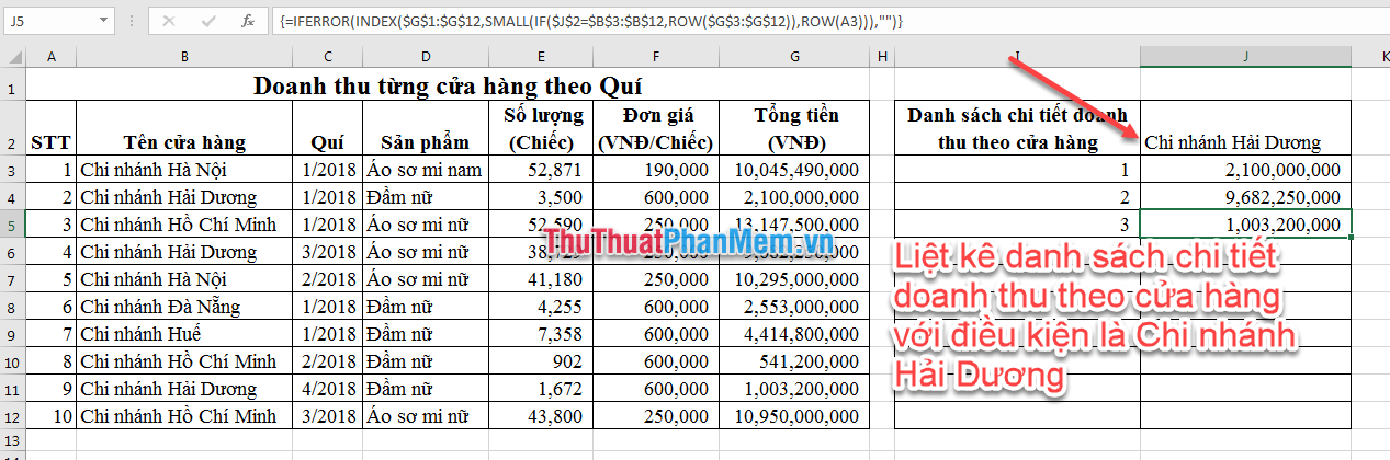
Consider the following example: You summarize data table and need to extract all data conditionally into another table.

How to list conditional lists in Excel Picture 2

So how can this be done? Today, the Software Dexterity will guide you how to combine the available functions to list all the conditional values ​​in Excel as functions: IFERROR, INDEX, SMALL .

IFERROR function

Function structure: = IFERROR (value, value_if_error) .

Inside:

- IFERROR : is the name of the function used to detect the error value and return the value you need.

- Value : The value we need to determine is an error or not.

- Value_if_error : return value if value is error.

If the value of the value is an error (# N / A, # REF, .), the IFERROR function will return the value_if_error , otherwise it will return a value value .

INDEX function

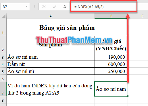
Function syntax: = INDEX (array, row_num, [column_num]) .

Inside:

- INDEX : is the name of the function used to retrieve the value in row n ( row_num) in the array data array .

- Array : Data array. In this article, the Software Tips only guide INDEX function with array as an array of data containing only one column.

- row_num : Select the row in the array from which to return a value.

Example of using the INDEX function:

How to list conditional lists in Excel Picture 3

SMALL function

Function syntax: = SMALL (array, k) .

Inside:

- SMALL : is the name of the function used to determine the smallest value k.

- Array: An array or range of numeric data that you want to determine its kth smallest value.

- K: Position (from the smallest value) in an array or range of data to return.

Example of using the SMALL function:

How to list conditional lists in Excel Picture 4

How to list conditional lists in Excel

With the requirement that Dexterity Software made above, you need to list 3 revenue items of Hai Duong Branch in column J.

In column J4 enter the formula: = IFERROR (INDEX ($ G $ 1: $ G $ 12, SMALL (IF ($ J $ 2 = $ B $ 3: $ B $ 12, ROW ($ G $ 3: $ G $ 12)), ROW (A1))), "") and press Ctrl + Shif + Enter . And copy the formula to other rows of columns.

How to list conditional lists in Excel Picture 5

Here:

1. $ G $ 1: $ G $ 12: is the reference data array to get the value to return.
2. $ J $ 2 is the position of the cell containing the value to search.
3. $ B $ 3: $ B $ 12 is the data array to be searched.

So based on the above formula, you change the position items of the data array and data cells corresponding to the position of your worksheet.

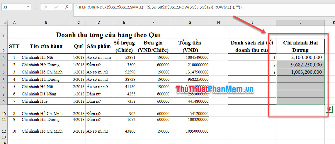
Note:

1. You should leave the absolute value of the data array to avoid errors when copying formulas.
2. If your reference range is long, you should copy the formula for the entire column or at least equal the number of rows of the reference range for safety. Ad has copied the formula until cell J9, but because only 3 search values ​​are satisfied that the Hai Duong Branch condition should only contain cells J3-J4 with numeric data, the other cells will be blank data. and will not affect the aesthetics of the report.

How to list conditional lists in Excel Picture 6

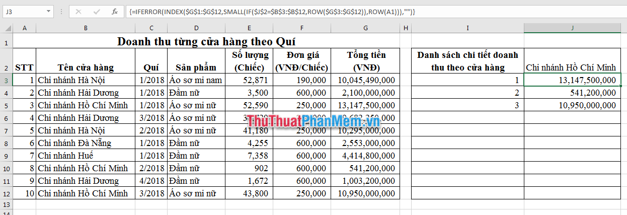
The image below is another result if the Dexterity Software changes the reference condition: Ho Chi Minh Branch.

How to list conditional lists in Excel Picture 7

Good luck!