How to format data in Excel

The following article details how to format commonly used data in Excel.

1. Steps to data formatting

Step 1: Select the data to format -> Right-click -> Select Format Cells .

How to format data in Excel Picture 1

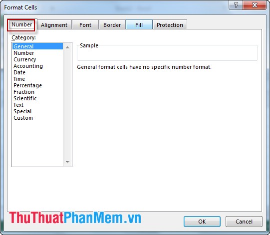
Step 2: A dialog box appears -> Choose the Number tab to choose the type of format.

How to format data in Excel Picture 2

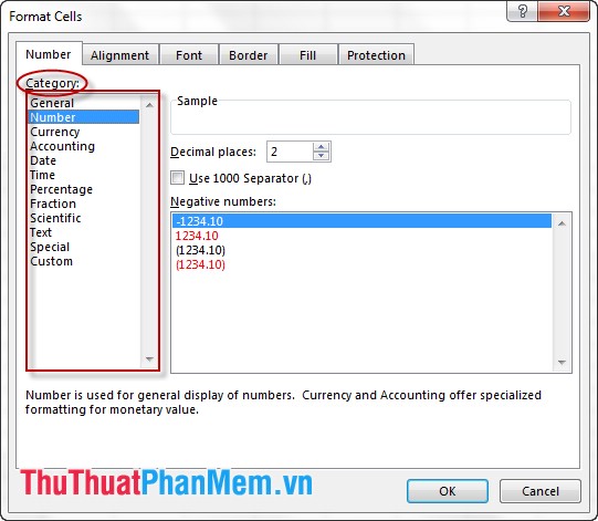
2. Select the data type

The data format is displayed in Category .

How to format data in Excel Picture 3

2.1. General format

The default format (which may be numbers or symbols .) case you have not selected a default Excel format General .

How to format data in Excel Picture 4

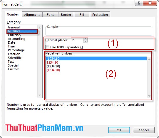
2.2. Number format

- Section Decimal places: the number of decimal places is displayed. You can make your own choice by clicking on the arrow.

- Item Use 1000 Sparator (,): Use commas separating thousands. If so, please tick.

- Negative Numbers: How to display numbers with negative values. There are 4 options as shown.

How to format data in Excel Picture 5

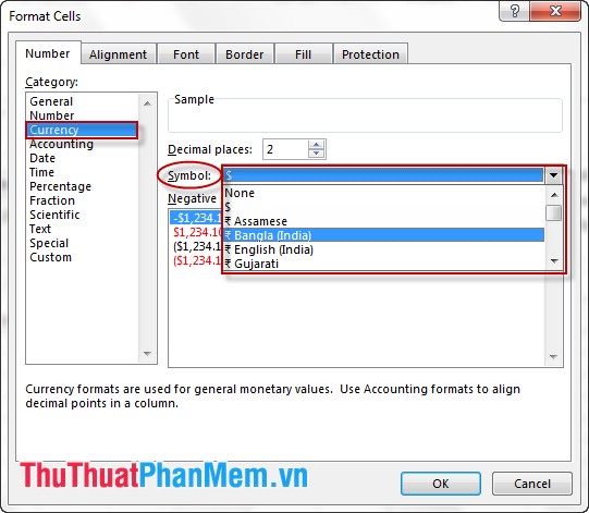
2.3. Currency Format: Format the currency type.

Like the Number format, the only difference is that it allows adding currencies to the left of the value, for example $ .

How to format data in Excel Picture 6

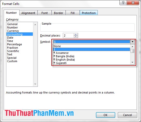
2.4. Accounting format

- Same as Currency format, only the currency unit is aligned with each other.

How to format data in Excel Picture 7

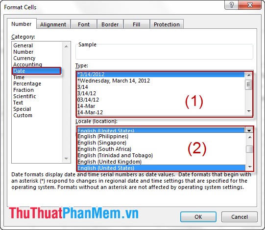
2.5. Date format

Item Type: Select display type: Date-> month-> year or date and month display . Lots of options for you.

Item Locale (location): you select the area to display the date.

Note: When you select the date, month and year format if you enter the wrong format, the machine will still return to the correct format of that data column.

How to format data in Excel Picture 8

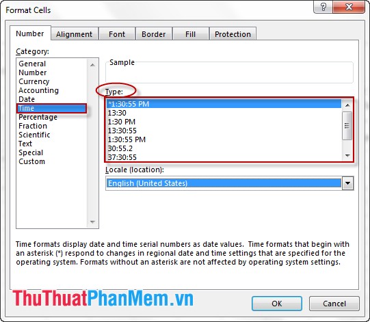
2.6. Time format

Allow users to enter time in many different formats. You choose the time display format in the Type section .

How to format data in Excel Picture 9

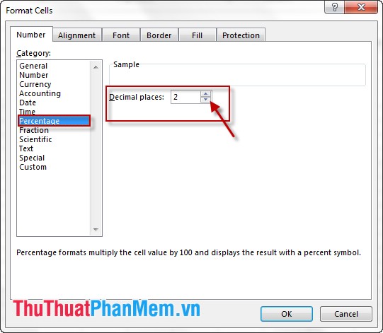
2.7. Percentage format

In percent format, select the number of decimal places shown in the Decimal Places section .

With this format, there is always a "%" sign after the number.

How to format data in Excel Picture 10

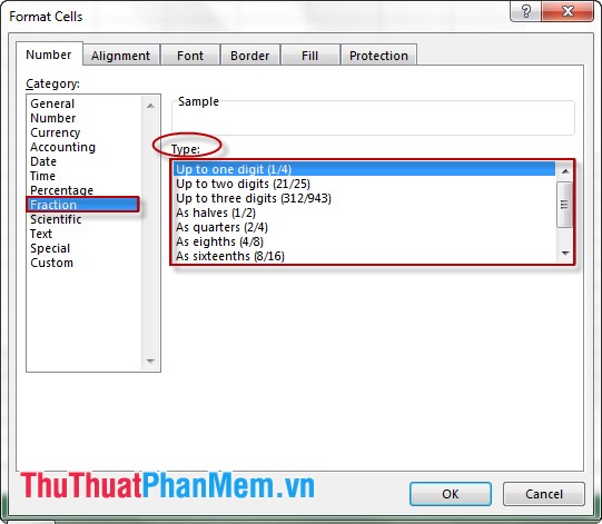
2.8. Fraction format

Fraction format allows users to choose the type of format to display in the Type section . There are many ways to display:

How to format data in Excel Picture 11

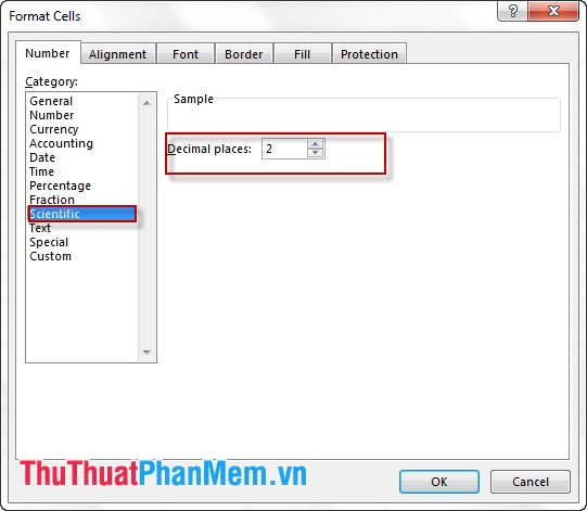
2.9. Scientific format

- Display numbers as exponents. For example:

2.00E + 0.5 = 200,000

2.05E + 0.5 = 205,000

- Choose the number of digits that displays after the dot in Decimal Places .

For example, choose value 1 => result 6.8E + 03

How to format data in Excel Picture 12

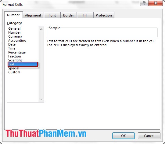
2.10. Text format

Format text style. Note that this range cannot be calculated even if you see them as numbers.

How to format data in Excel Picture 13

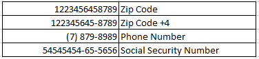
2.11. Special format

Special types of phone numbers.

Choose the type of display in the Type section , there are 4 types of options.

How to format data in Excel Picture 14

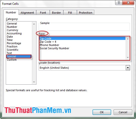
For example: 4 types of phone number formats.

How to format data in Excel Picture 15

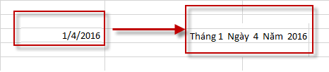
2.12. Custom format

User-defined formats may be based on available formats. For example, based on the format "m / d / yyyy" may have the format "Month m Day d Year yyy" by entering the Type as shown.

How to format data in Excel Picture 16

After completing the import, you have the following result:

How to format data in Excel Picture 17

Good luck!