Instructions on how to format data in Excel

The following article details you how to format data in Excel 2013.

1. Format text.

1.1 Font format, type, font size:

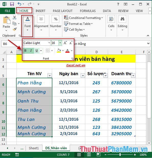
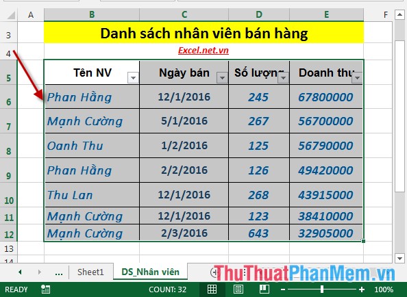
- Select the data to format -> Home -> Font -> quickly select the font, font size, type as shown:

Inside:

+ B (Bold): bold type.

+ I (Italic): italic type.

+ U (Underline): underlined font

Instructions on how to format data in Excel Picture 1

- Or to detail Font dialog box, click the arrow below Font -> Format Cells dialog box appears, select the format for the text -> click OK to finish.

Instructions on how to format data in Excel Picture 2

1.2 Border format, text color.

1.2.1 Select text color and background color:

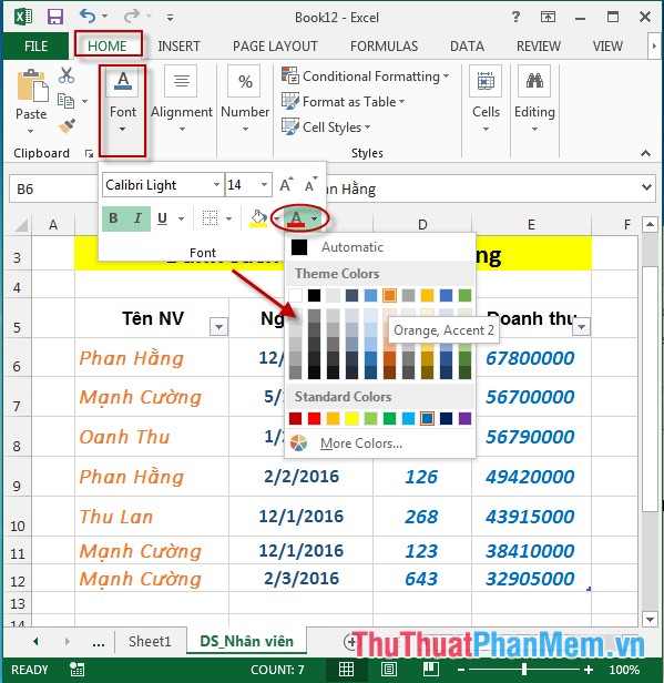
- Select the text area to create colors -> Click Home -> Font -> select the Font Color icon -> dialog box appears -> choose the color for text:

Instructions on how to format data in Excel Picture 3

- Select background color for text:

Select the text area to create background color -> Click Home -> Font -> select the Fill Color icon -> dialog box appears -> select the color as the background color for the text:

Instructions on how to format data in Excel Picture 4

- Result:

Instructions on how to format data in Excel Picture 5

1.1.2 Create borders for text:

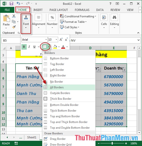
Click Home -> Font -> select Border icon -> dialog box appears -> choose the border style for the text:

Instructions on how to format data in Excel Picture 6

- The result of the entire text has been created contour:

Instructions on how to format data in Excel Picture 7

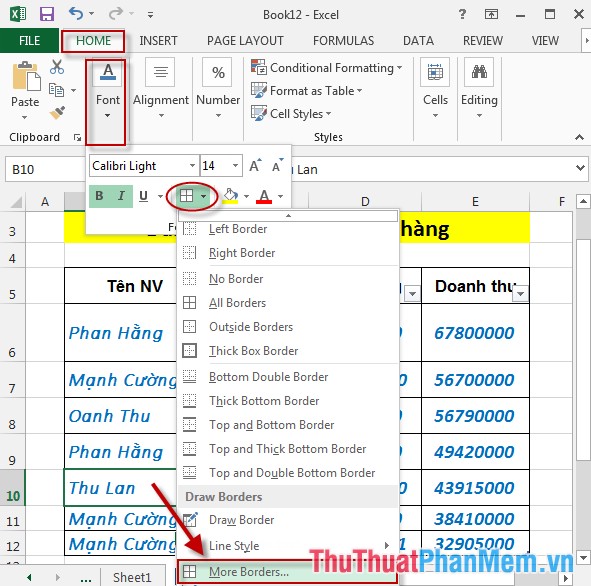
- If you want to create a border as you like Click Home -> Font -> select Border icon -> dialog box appears -> More Border:

Instructions on how to format data in Excel Picture 8

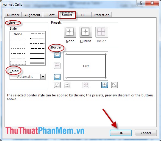
- The dialog box appears selecting the type of border, colors as shown -> click OK:

Instructions on how to format data in Excel Picture 9

2. Align, customize position, text direction.

2.1 Alignments.

- Select text area to be aligned -> Click Home -> Alignment -> choose alignment:

Instructions on how to format data in Excel Picture 10 : Aligns the left.

Instructions on how to format data in Excel Picture 11 : Align justify sides.

Instructions on how to format data in Excel Picture 12 : Right alignment.

Instructions on how to format data in Excel Picture 13

2.2 Customize text position in cell.

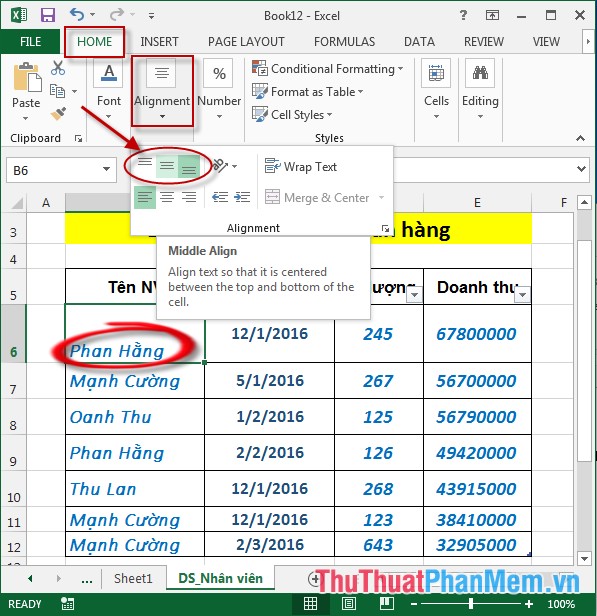
- If the data cell is too wide for the text to align the text so that it is in the middle and proportional to the data cell -> align the position of the text in the cell, there are options such as the figure:

Instructions on how to format data in Excel Picture 14 : The order in turn is: Align the text adjacent to the top of the cell (top), center the cell, and the text position at the end of the cell.

Instructions on how to format data in Excel Picture 15

- Or you can align in the Format Cells dialog box :

Instructions on how to format data in Excel Picture 16

- Click OK to get the results: The text in the middle of the cell is very balanced.

Instructions on how to format data in Excel Picture 17

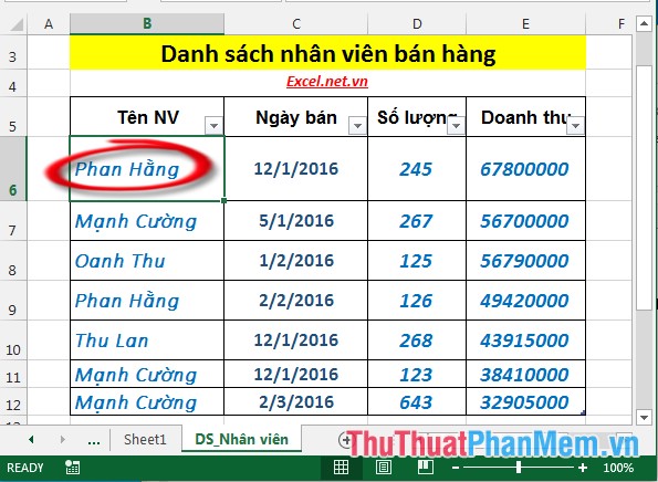
2.3. Customize the text direction.

- Select the text to create text direction -> Click Home -> Alignment -> Orientation -> select text direction as required.

Instructions on how to format data in Excel Picture 18

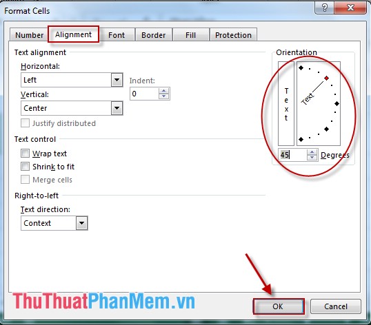
- Or change the text direction in the Format Cells dialog box in the Alignment tab :

Instructions on how to format data in Excel Picture 19

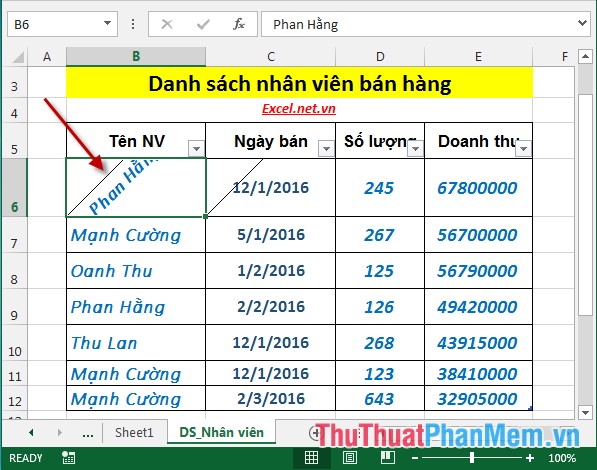
- Results after creating the letter direction:

Instructions on how to format data in Excel Picture 20

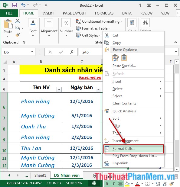
3. Format the data type.

- For example, you want to format the column number data type to date data type:

Instructions on how to format data in Excel Picture 21

- Right-click the column of quantities -> Format Cells:

Instructions on how to format data in Excel Picture 22

- The Format Cells dialog box appears in the Number tab, selecting the Date data type .

Instructions on how to format data in Excel Picture 23

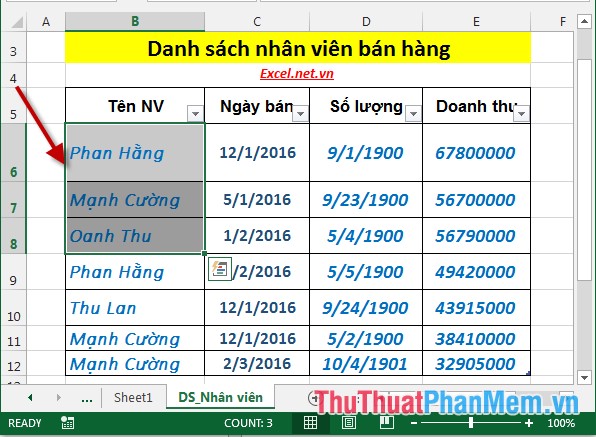
- Result of the column of the converted date data type:

Instructions on how to format data in Excel Picture 24

The above is a detailed guide on how to format data in Excel 2013.

Good luck!