Instructions to stamp negative numbers in Excel

When performing data calculations on Excel, we will have to work with different types of numbers. And in the data table, you have the need to distinguish negative numbers with other types of numbers, making it easier to perform more operations that can be closed in parentheses, or even reded if there are negative numbers. In the article below, Network Administrator will guide you how to close brackets and blacken negative numbers in Excel.

Video tutorial to create brackets with negative Excel numbers

How to create brackets for negative numbers on Excel

Step 1:

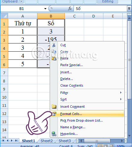
First of all, we will draw the data table and enter the number in the table with negative numbers. Next, black out the column or area that needs negative number format with parentheses or redheads. Next right click on the blacked area and select Format Cells .

Instructions to stamp negative numbers in Excel Picture 1

Step 2:

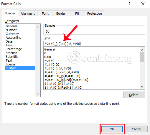
Appearance of Format Cells window interface. Select the Number tab . Here, the Category section we will select Custom . Look to the right of the Type item, you will find the format #, ## 0 _); (#, ## 0) , and then click OK to use.

Instructions to stamp negative numbers in Excel Picture 2

Step 3:

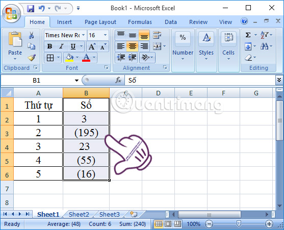
Immediately afterwards, all negative numbers in the data sheet will be enclosed in brackets and lose the sign - as before as shown below.

Instructions to stamp negative numbers in Excel Picture 3

Step 4:

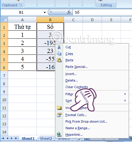
Next, if you want to redirect negative numbers in the data table and still keep the - in front , we also highlight the area you want to format and right-click and choose Format Cells .

Instructions to stamp negative numbers in Excel Picture 4

Step 5:

Also at the Number item Custom tab, we will find the format #, ## 0 _), [Red] (- #, ## 0) in the Type section. Click OK to proceed.

Note , if in the Type section of the Excel version is not available, we can copy and paste that format into Type and click OK to apply.

Instructions to stamp negative numbers in Excel Picture 5

Immediately after that, the negative number in the data sheet has been converted to the closed and redened format as shown below.

Instructions to stamp negative numbers in Excel Picture 6

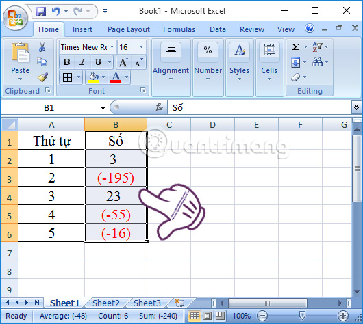
Above are 2 ways to format negative numbers in data tables on Excel. With this method, you can easily identify negative numbers in the data sheet, making data manipulation easier.

Refer to the following articles:

1. Summary of expensive shortcuts in Microsoft Excel
2. These are the most basic functions in Excel that you need to understand
3. Instructions for printing two-sided paper in Word, PDF, Excel

I wish you all success!