How to format numbers in Excel

In the process of working, processing data in Excel sometimes you need to format numbers in Excel so that data can display the number format in accordance with the requirements to be processed. You do not know how to format numbers in Excel so you can fit what you need. So, please refer to the following article to know how to format numbers in Excel.

How to format numbers in Excel Picture 1

Here's how to format numbers in Excel, please follow along.

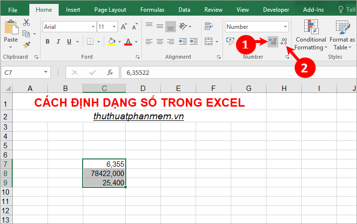
Method 1: Format the number in the Number section of the Home tab.

Select the cells you need to format numbers, on the Home tab you look for the Number . Next you choose Number in the format box.

How to format numbers in Excel Picture 2

To increase or decrease the number of digits after the decimal point, you select the symbol (1) if you want to increase the number of digits after the decimal point, select (2) if you want to reduce the number of digits after the decimal point stool.

How to format numbers in Excel Picture 3

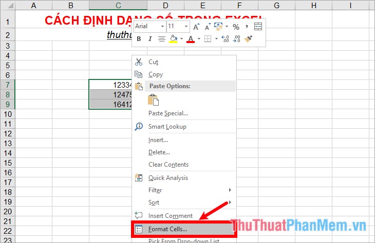
Method 2: Format numbers using Format Cells

Step 1 : Select the cells to format, right-click and select Format Cells or press Ctrl + 1 to open the Format Cells dialog box .

How to format numbers in Excel Picture 4

Step 2: The Format Cells dialog box appears , on the Number tab, select Number in the Category section to select the number format in Excel. In the right side, select or enter the number of words after the decimal point in the Decimal places box . If you want to use dots to separate 1000, then tick the box before Use 1000 Separator (.).

How to format numbers in Excel Picture 5

In the Negative numbers section, you can choose the type of display for negative numbers, if it is negative, remove negative signs and numbers to red, then select the corresponding type as shown below (you can choose the negative number type) other you want).

How to format numbers in Excel Picture 6

If the cell you choose to format the number has been entered, the first number in the area you select will be displayed preview in the Sample section , if you find it inappropriate you can edit accordingly. After the number format is complete, click OK to close Format Cells.

How to format numbers in Excel Picture 7

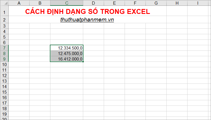
So the area you have chosen is formatted as what you have set.

How to format numbers in Excel Picture 8

Custom number format

If you want to format the custom number display format yourself, do the following:

First, you also select the data range to be formatted and press Ctrl + 1 to open Format Cells .

How to format numbers in Excel Picture 9

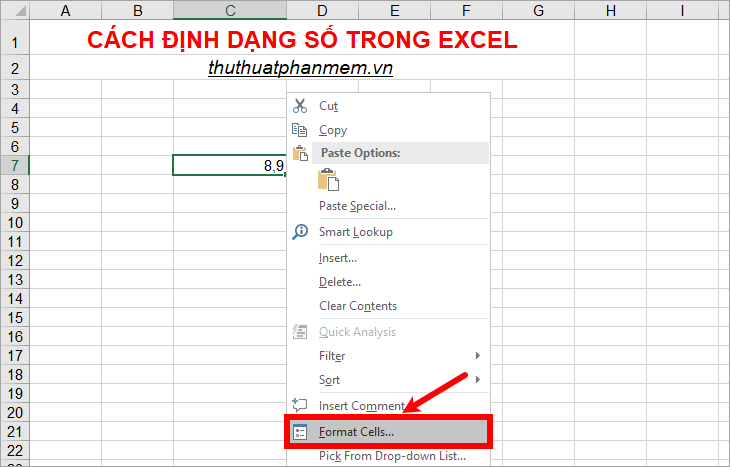
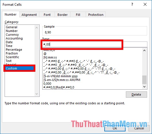
On the Number tab of Format Cells, select Custom and enter the custom format you want in the box below Type .

For example, you want to display the last zero if the number doesn't have 2 digits after the decimal point. As when entering the number 8.9 you want to display is 8.90, then you enter the custom format is #, 00. Thus the number will be displayed as you desire.

How to format numbers in Excel Picture 10

So, above article has shared with you how to format numbers in Excel. Hopefully through this article, you will be able to better understand how to format numbers in Excel so you can apply the number format to suit the requirements that you need to handle. Good luck!