Instructions for formatting data in Excel

Excel spreadsheets support a variety of data types for cells in the worksheet: numeric, percentage, date, time, fraction, etc., with different data, you should format the data type correctly. for that data box. Thus when calculating or processing data will be easier and more accurate.

The default data type in Excel spreadsheets is always the General format. You can change the data type format in Excel with the following steps:

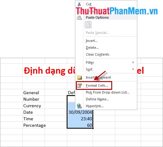
Step 1: Select the data cells to format, then right-click -> Format Cells .

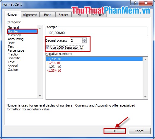
Step 2: In Format Cells , in the Number tab there are many formats in the Category section .

General: The default default Excel type when you type.

Number: Formats a numeric data format.

Currency and Accounting: is the format for currency data.

Date: The format for the date data type.

Time: Format the time type for data.

Percentage: Format the percentage type for data.

Fraction: Fractional data format.

Scientific: Abbreviated numeric data format

Text: Typographic data format.

Special: Special data format.

Custom: The type of user to format themselves.

Step 3: Format the data according to some commonly used types

- If you format the numeric data, select the Number type in the Category. In the Decimal places section, you choose the number of digits after the comma, or you want to add the "," as a separator for numbers if they have a value of thousands of units, then check the box before Use 1000 Sepatator (,). Then click OK .

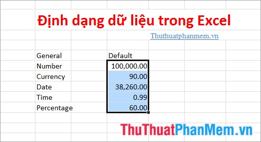
The result after setting the data as Number.

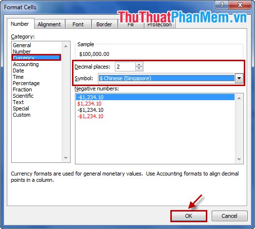
- If you want to format the data type of currency, in Format Cells, select Currency in Category. Select the number of digits after the comma in Decimal places and select the type of the currency symbol for the data in Symbol and then click OK .

And the result if choosing the currency type for the data:

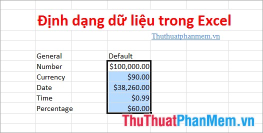
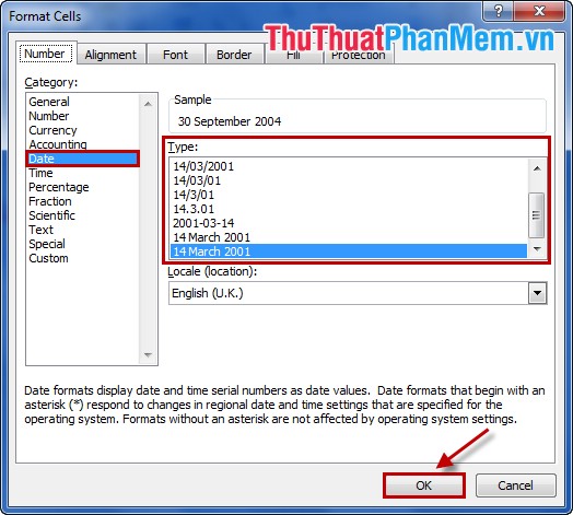
- If you format the date format, then in Format Cells you select Date in Category. Next you choose the date format in the Type section and then click OK .

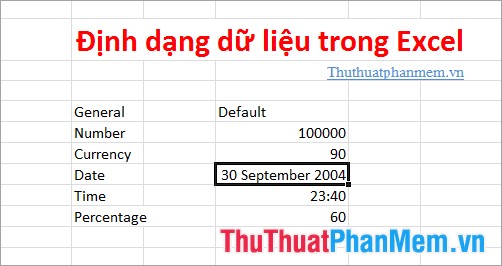
The result after making the date format.

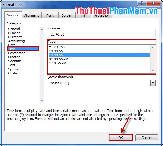
- If you format the data according to the time format, in Format Cells you select the Time type in Category, select the time format in the Type section and click OK .

After selecting the time format, the results are as follows:

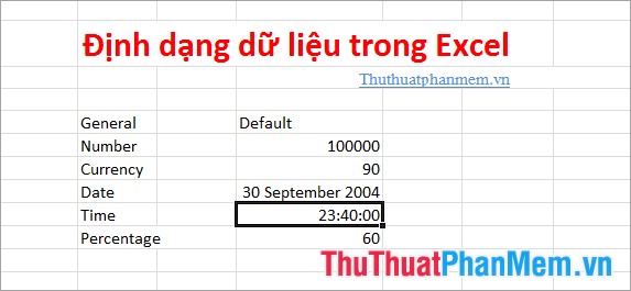
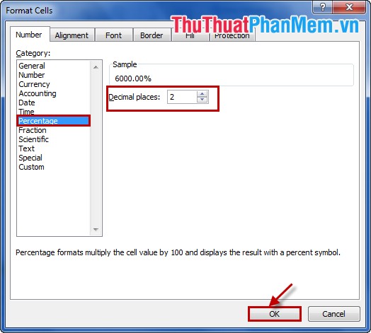
- If you format the data as a percentage, in Format Cells, select Percentage in Category and select the number of digits after the comma in Decimal places. Then click OK .

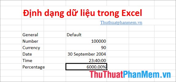
The result will look like this:

With other data types, you also do the same thing to choose the right data format format that suits the data cell.

So, you already know how to format data in Excel spreadsheets. Good luck!