Guide to full Excel 2016 (Part 7): Format spreadsheet data

1. A complete guide to Excel 2016 (Part 4): How to store and share spreadsheets
2. Complete tutorial of Excel 2016 (Part 5): Basics of cells and ranges
3. Complete tutorial of Excel 2016 (Part 6): Change the size of columns, rows and cells

If you have seen the article about Microsoft Word, then you also have some basic knowledge about text alignment. Because we work with spreadsheets primarily as a calculation, we don't need too much alignment, but it should be enough for others to see tables that can capture its structure. Please refer to the article of formatting spreadsheet data in Excel 2016 in this article!

A. Introduction

All cell content uses the same format by default, which can make it difficult to read a spreadsheet. The basic format can customize the look and feel of the spreadsheet, allowing you to draw attention to specific sections and make your content easier to see and understand.

See the video below to learn more about cell formatting in Excel 2016 :

I. Change font size:

1. Select the cell (s) you want to modify.

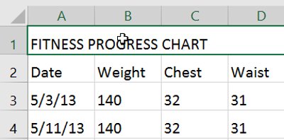
2. On the Home tab, click the drop-down arrow next to the Font Size command, then select the desired font size. In the example, we select the 24 font to make the text clearer.

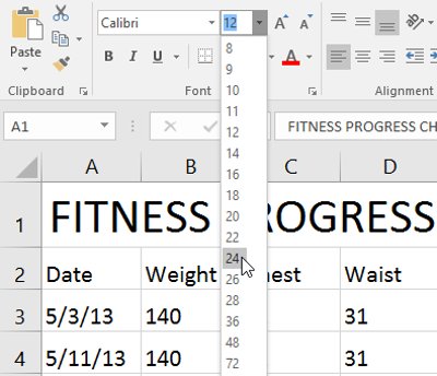
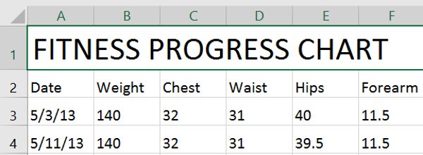
3. Text will change the selected font size.

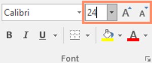
1. You can also use the Increase Font Size and Decrease Font Size commands or enter a custom font size using the keyboard.

II. Change fonts:

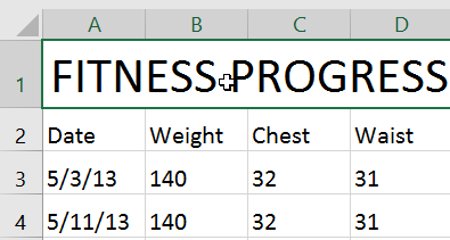
By default, the font of each spreadsheet is set to Calibri . However, Excel 2016 provides many other fonts you can use to customize your cell text. In the example below, we format the title box to help distinguish it from the rest of the spreadsheet.

1. Select the cell (s) you want to modify.

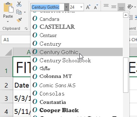
2. On the Home tab, click the drop-down arrow next to the Font command, then select the font you want. In the example, we chose Century Gothic .

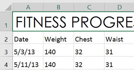
3. The text will change to the selected font.

1. When creating a workbook in the workplace, you will want to choose an easy-to-read font. Along with Calibri , standard readable fonts include Cambria , Times New Roman and Arial .

III. Change font color:

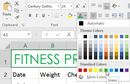
1. Select the cell (s) you want to modify.

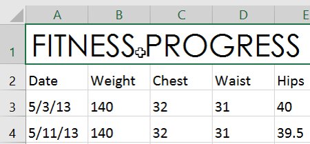
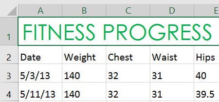
2. On the Home tab, click the drop-down arrow next to the Font Color command, then select the desired font color. In the example, we will choose green.

3. The text will change the selected font color.

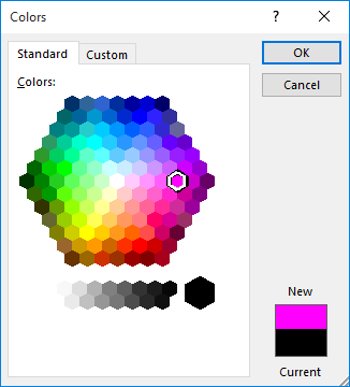
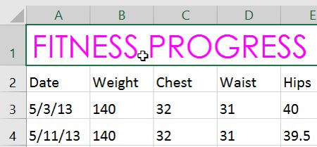
1. Select More Colors at the bottom of the menu to access additional color options. We changed the font color to bright pink.

B. Use Bold commands (Bold), Italic (Tilt) and Underline (Underline):

1. Select the cell (s) you want to modify.

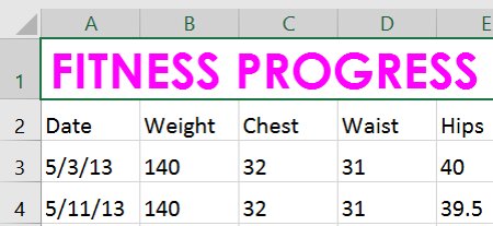
2. Click the Bold ( B ), Italic ( I ) or Underline ( U ) command on the Home tab. In the example, we make the selected cells bold.

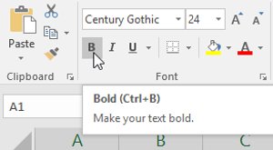
3. The type you selected will apply to the text.

1. In addition, you can also press Ctrl + B on the keyboard to make bold text, Ctrl + I to tilt the text and Ctrl + U to underline.

C. Cell border and fill color

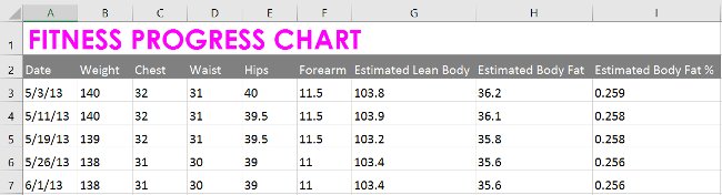
Borders and shading allow you to create clear and defined boundaries for different parts of the spreadsheet. Below, we'll add borders and color to the title boxes to help distinguish them from the rest of the spreadsheet.

I. Add color:

1. Select the cell (s) you want to modify.

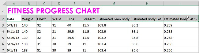
2. On the Home tab, click the drop-down arrow next to the Fill Color command, then select the fill color you want to use. In the example, we will choose dark gray.

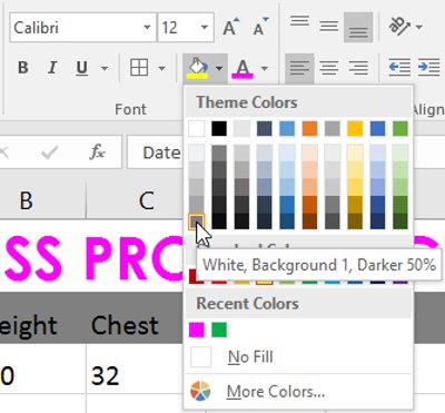
3. The color will appear in the selected cells. We have also changed the background color to white to make it readable with darker colors.

II. Add a border:

1. Select the cell (s) you want to modify.

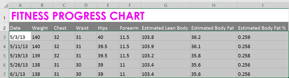
2. On the Home tab, click the drop-down arrow next to the Borders command, then select the type of border you want to use. In the example, we will choose to display All Borders .

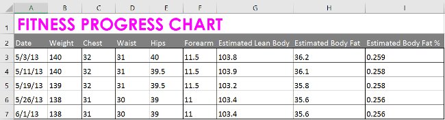
3. The selected border will appear.

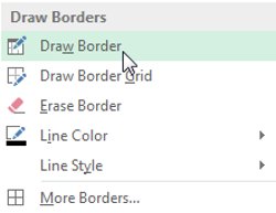
1. You can draw borders and change the border styles and colors of borders with the Draw Borders tool at the bottom of the Borders drop-down menu.

1. 4 basic steps to color alternating columns in Microsoft Excel

D. Cell styles

Instead of manually formatting cells, you can use Excel 2016 predefined Cell styles. Cell style is a quick way to include professional formats for different parts of spreadsheet, such as the title of the article and the page title.

Apply cell style

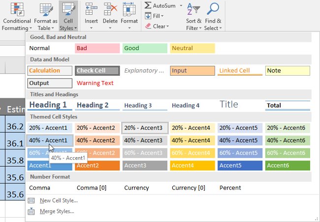
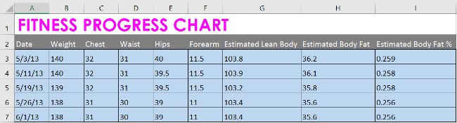
In our example, we will apply a new cell style to the current cell title and title.

1. Select the cell (s) you want to modify.

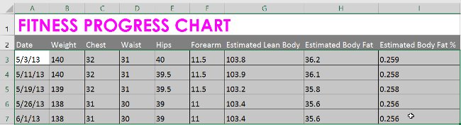
2. Click on the cell type on the cell style tab, then select the desired type from the drop-down menu.

3. The selected cell style will appear.

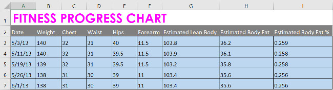
1. Applying cell style will replace any existing cell format except text alignment. You may not want to use cell styles if you have added more formats to your spreadsheet.

E. Align margins for data

By default, any text entered into your spreadsheet will be aligned to the bottom left of a cell, while any number will be aligned to the bottom right. Changing the cell content alignment allows you to choose how content is displayed in any cell, which can make your cell content more readable.

1. Left Align : Left alignment.

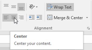
1. Center Align : Center alignment.

1. Right Align : Right alignment.

1. Top Align : Align the content with the top border of the cell.

1. Middle Align : Center the content with equal distance from top to bottom and bottom of the cell

1. Bottom Align : Align the content with the bottom border of the cell.

I. Horizontal alignment (Horizontal) of the cell:

In the example below, we will modify the layout of the title box to create a more refined and clear view from the rest of the spreadsheet.

1. Select the cell (s) you want to modify.

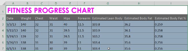
2. Select one of three horizontal alignment commands on the Home tab. In the example, we will select Center Align .

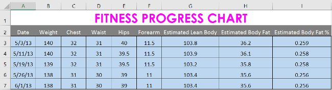
3. The text will be re-aligned.

II. Align vertical (Vertical) of the cell:

1. Select the cell (s) you want to modify.

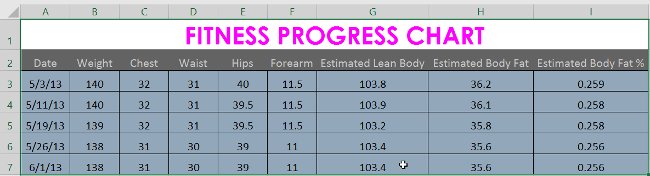
2. Choose one of the three vertical alignment commands on the Home tab. In the example, we will select Middle Align (Center the content vertically ).

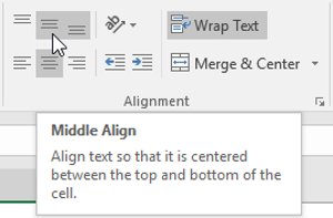
3. The text will be re-aligned.

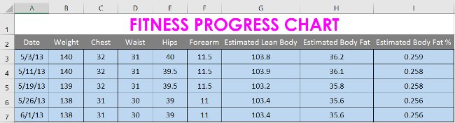
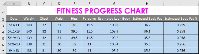
1. You can apply both vertical and horizontal alignment to any cell in the spreadsheet.

F. Format Painter

If you want to copy the format from one cell to another, you can use the Format Painter command on the Home tab. When you click Format Painter, it will copy all formats from the selected cells. You can then click and drag over any box you want to paste the format into.

Watch the video below to learn about two different ways to use Format Painter :

See also: Complete guide to Excel 2016 (Part 1): Get familiar with Microsoft Excel

Next lesson: Complete guide to Excel 2016 (Part 8): Learn about Number Formats

Having fun!