Filter PivotTable report data in Excel

The following article details you how to filter PivotTable reports data in Excel 2013 accurately and quickly.

The original PivotTable report created on demand helps you see the entire information of the data. In case you want to statistic data by a certain field, you can use the data filtering method to know exactly what information you are looking for.

You have created a complete report:

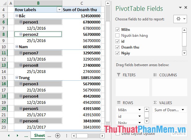
But due to work requirements you need to statistically follow a number of criteria to give sales direction -> use the data filtering feature in the PivotTable.

1. Filter to see 1 in many sales people.

For example, to filter the report data by salespeople, and these employees are sorted by descending order of sales by default.

Step 1: Right-click on the vendor's field name -> Add to Report Filter.

Step 2: After selecting the field to filter -> the data in the report varies by salesperson, and the sales field is added to the FILTERS filter list .

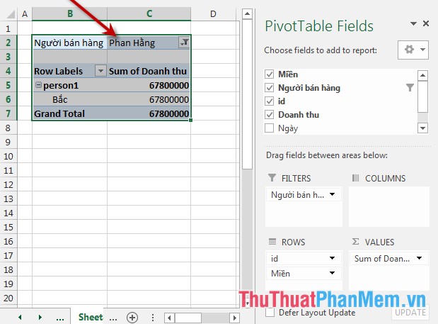
Step 3: Now you want to display detailed information about a certain salesperson, do the following: Move to the top of the report click on the arrow -> list of displayed employees -> select Name of employee want to know information -> Click OK.

Step 4: After clicking OK -> all employee details are displayed:

- If you want to display all employees instead of clicking the employee name, click All.

2. Find out salespeople who have high sales in the data sheet.

Step 1: Add the revenue field to the ROWS dialog box by: Right-clicking the field name -> selecting Add to Row labels.

Step 2: Click the arrow in Row Labels -> Value Filters -> Greater Than Or Equal To (or you can choose a different arrangement depending on your purpose):

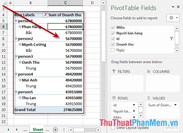
Step 3: The Value Filter (id) dialog box appears to enter the value to compare. For example, here find employees with sales greater than or equal to 4391500 -> click OK.

After selecting OK -> employees with sales greater than or equal to 43915000 are displayed on the report, those employees with smaller sales are not displayed.

3. Filter information over time.

To filter information over time you need to pay attention to the following:

+ Date data types must be formatted as dates supported by Excel 2013.

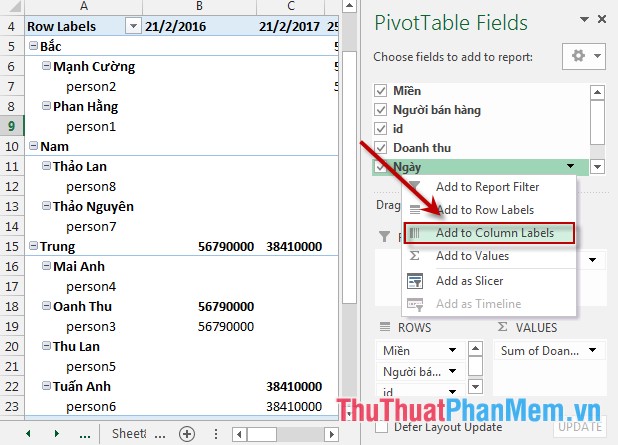
+ Should add date field to the column for science.

Step 1: Right-click the date field -> Add to Column Labels:

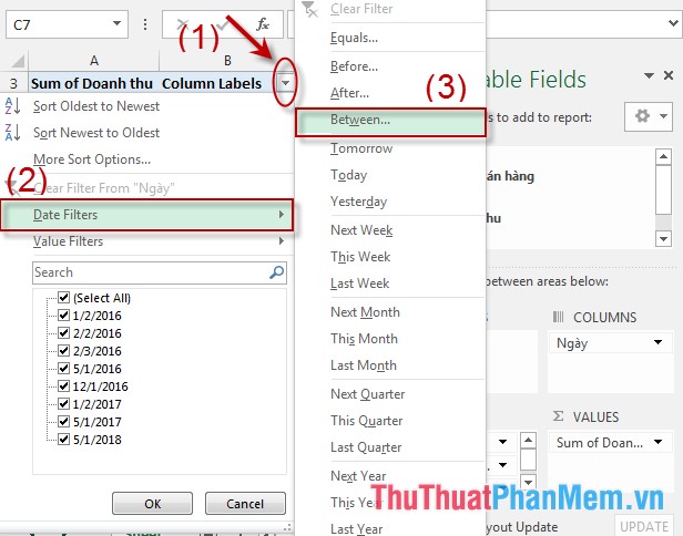
Step 2: Click the arrow of Column Labels -> Date Filters -> Between (or you can choose another type of comparison depending on the purpose):

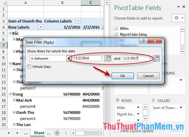
Step 3: Enter the date value in the period you want to statistic -> click OK:

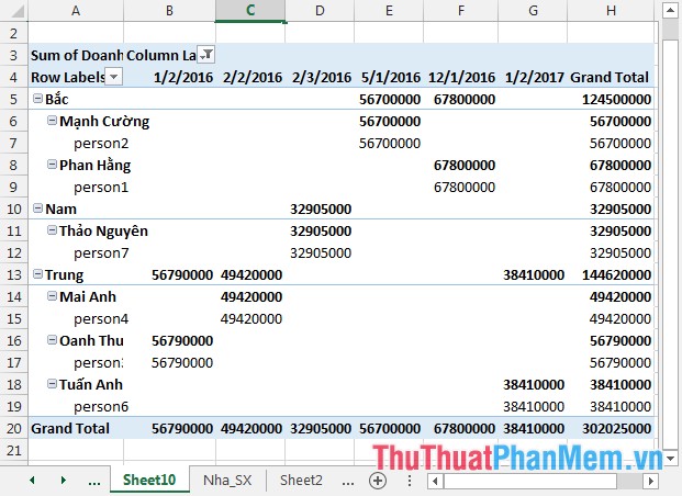
- After clicking OK the results:

4. Remove filters.

To remove the filter, you need to delete both parts of the PivotTable reports.

- Delete a filter in a PivotTable:

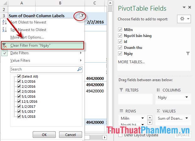
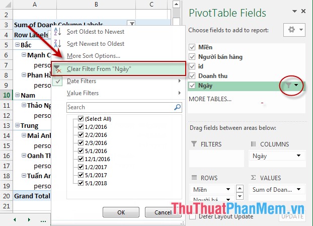
With the filter by row or column similar operation: Click on the arrow icon Column Labels -> Clear Filter From 'Date'

- Delete filters in PivotTable Filed List:

Click on the filter icon next to the field name -> Clear Filter From 'Date'

With the above two actions, you have removed the filter in the PivotTable.

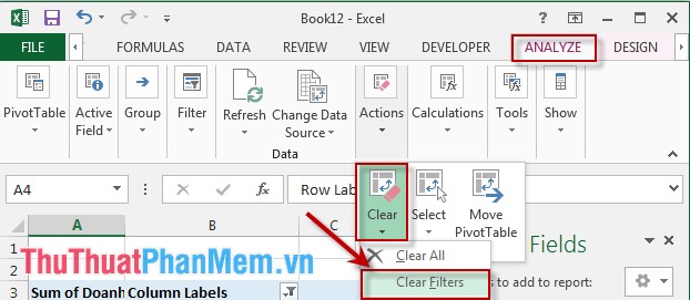
5. Remove 1 filter in the PivotTable report.

If you do not find Clear Filter From to cancel the filter in Filter or you want to delete all filters in the PivotTable do the following: Click on the PivotTable -> move to ANALYZE -> Action -> Clear - > Clear Filters:

Above is a detailed guide on how to filter data in a PivotTable in Excel 2013.

Good luck!