How to Hide Formulas in Excel

This practical guide walks through how to hide formulas in Excel, explains the main requirements, and highlights common issues that may appear along the way.

Instructions for hiding Excel formulas

Step 1:

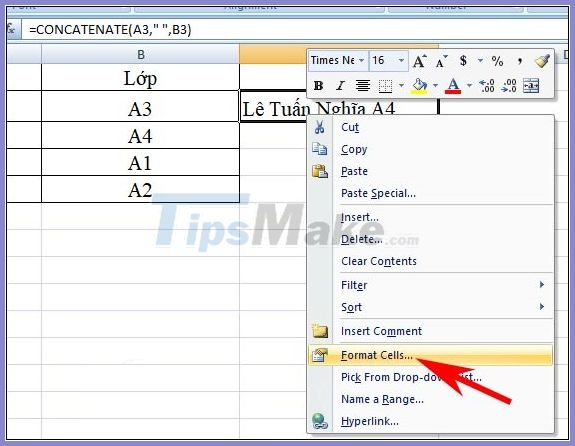
In the Excel data sheet interface, click on the formula cell you want to hide in the data table, then right-click and select Format Cells in the displayed list.

Step 2:

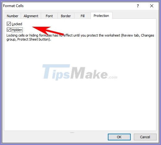
In the new interface displayed, click the Protection tab and then click the Hidden check box . Click OK to save.

Step 3:

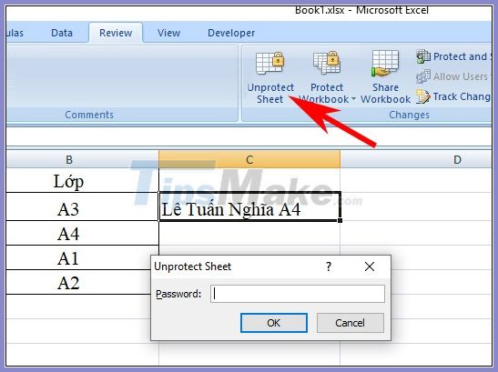
Back to the Excel interface, click the Review tab and select Protect Sheet . Now display a new interface, enter the password at Password to unprotect sheet . Click OK and re-enter the password.

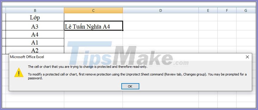
The result when you click on the formula cell disappears and only displays the result. When clicked also cannot edit the content and is reported as shown below.

Step 4:

To unhide the formula cell, click the Review tab > Unprotect Sheets again . Finally, you can enter the correct formula key password set up earlier. Right Then, the formula cell will display again as it was originally.