How to compare data on 2 columns in an Excel file

To compare data on two columns in Excel file we will use Excel's Conditional Formating function. But for you to better understand its principle mechanism, TipsMake.com will guide you step by step.

We will now familiarize ourselves with this issue with the following example. Compare the two columns of inventory name name data on day 1 and day 2 to see if any orders are repeated or not.

To do this we need to use the COUNTIF function . The COUNTIF function is a count function based on the conditions we set. The formula for the COUNTIF function is:

= COUNTIF (array of data to be counted, different conditions to count)

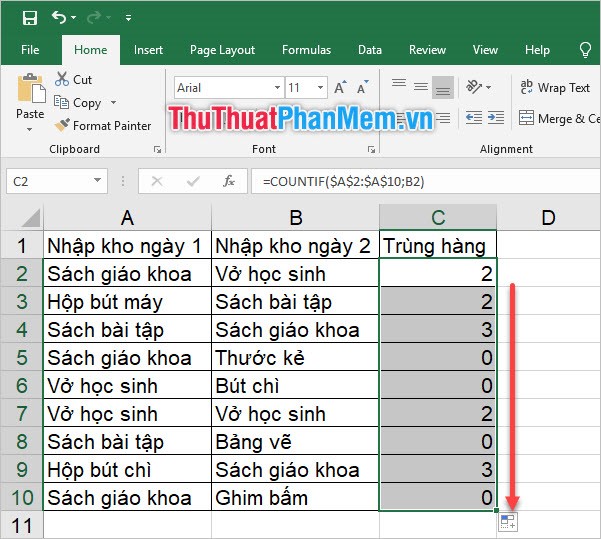
Here we need to compare the lines one by one so on the first line we will try to count whether "Student notebook" - the first item of the 2nd day of inventory has any coincidence with the first day or not.

So we have the following formula:

= COUNTIF (A2: A10; B2)

And don't forget to press F4 after the A2: A10 array to make it $ A $ 2: $ A $ 10 . This helps to fix the array, when we copy the formula later, it will not convert the number of rows according to the copy.

Place the mouse in the lower right corner of the formula cell then drag it down to copy the formula down.

If you click on the formula in one of the cells below, you will see that the "condition" element at the back will no longer be the B2 cell address as at the beginning because now when we copy down below, Excel will automatically increase the number of rows with the corresponding unit to transform according to the data of each row.

For example, in row 8, the condition part will be B8, in this row we will compare "The drawing board" with the "Inventory Day 1" array rather than the "Notebook" as before.

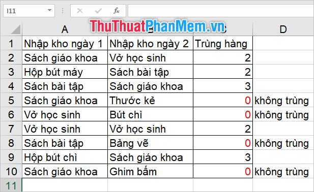
Now look at the table below and the results you will get after using the COUNTIF formula mentioned above. You can see that there will be a row of 0, which means that Excel does not count the value that matches the condition, or in other words it does not find any item in the Inventory on day 1 that coincides with the item at Warehouse 2 on the day, it means there is no match.

The remaining non-uniform numbers are the number of duplicate items.

If you now understand the principles of the COUNTIF formula above, let's learn about the problem that TipsMake.com mentioned at the beginning of this article: Conditional Formating .

First copy the COUNTIF formula again, because below it will be the core for your use of Conditional Formating .

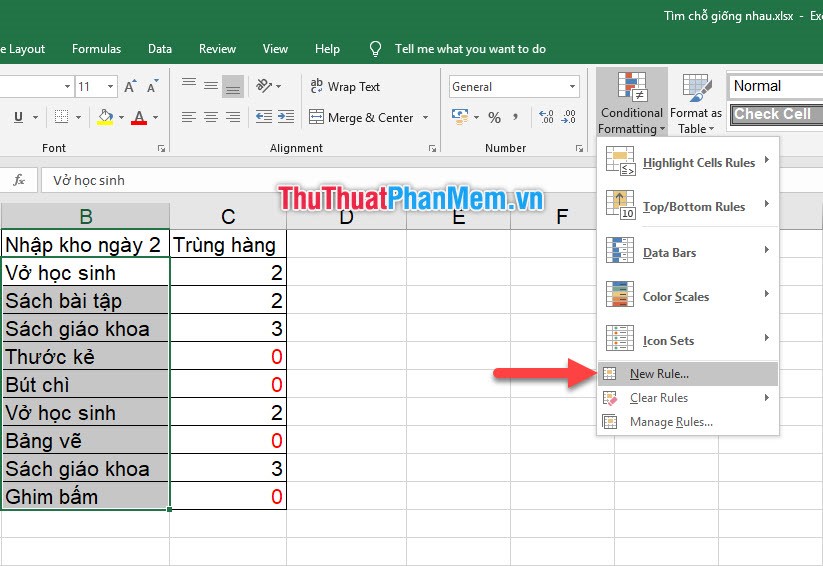
Highlight a column to compare data, then go to the Home ribbon in the toolbar. You will find items Styles with Conditional formating that we are looking for.

The Conditional Formating function helps you to change the format of your data cell based on a condition you set (normally people will use it to color cells that match the condition, making a difference with the cells. not suitable for other conditions). Here we will try to color blue for all the cells in the Day 2 Warehouse that have duplicates compared to the 1st Day Warehouse.

Because our conditional function is based on the COUNTIF function, which is quite special and different from the regular Conditional Formating color types , you have to choose New Rule to create your own coloring conditions.

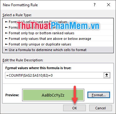
In the New Formating Rule function dialog box , click on the Rule a formula to determine which cells to format line .

Then in the empty Format values ​​where this formula is true (format the cells with the following formula), paste the copied COUNTIF formula above.

Based on the principle we mentioned above with the COUNTIF formula , if the result is zero with this formula, we will get the "no duplication" of the two dates of entry. Therefore, we need to add = 0 in the back to find the results that the COUNTIF formula produces 0.

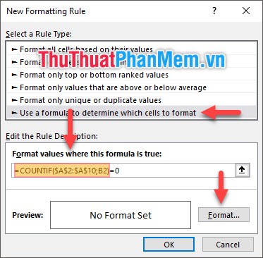
Do not forget to adjust the format created for the data cells in accordance with the condition by clicking Format . Because we only need to fill the data cell with green color, please click on the Fill tab and select the blue color and click OK .

Finally, click OK to confirm the setting to create a green consistent format for non-duplicated data cells.

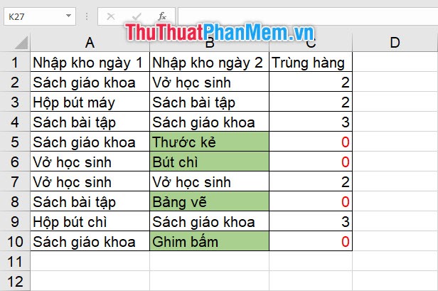
The result you get will be similar to the image below, the non-duplicate data cells will be highlighted in green, including: Ruler , Pencil , Drawing Board , Stapler .

To ensure aesthetics and no redundancy in Excel, you probably won't have an extra column just to count duplicates, so the COUNTIF formula in Format values ​​where this formula is true above. is necessary. But if you leave the COUNTIF row blank , then when writing the formula for Format values ​​where this formula is true , you only need to write = C2 = 0 . And so we will be based on the results COUNTIF has created outside.

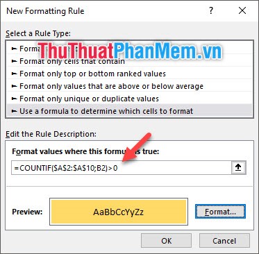
Similarly, if you change the operation in Format values ​​where this formula is true from = 0 to> 0, this will create the format for the cells containing the same data between the two dates.

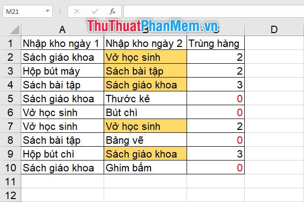
And the result is that the cells with the same data will be formatted exactly as you installed.

Thank you for following our article TipsMake.com on how to compare data on 2 columns in Excel file. Hopefully the article has given you more useful knowledge on how to compare data. We also have many other articles about software tips that you will definitely be interested in, please visit our homepage at TipsMake.com.