Steps to create graphs (charts) in Excel

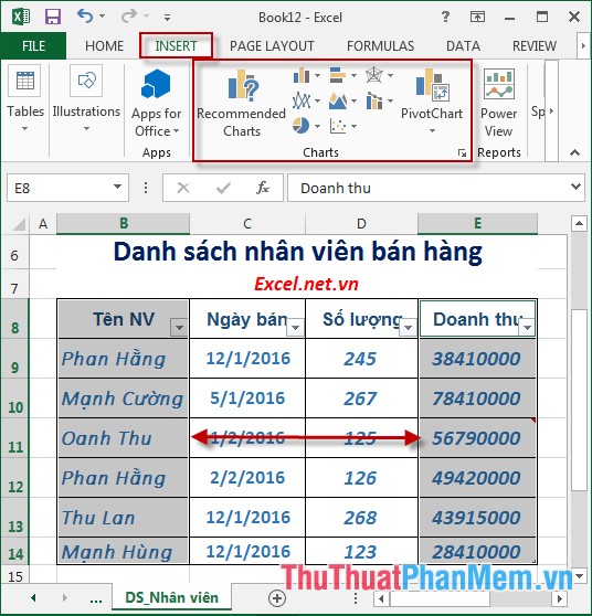
The following article gives detailed instructions for you to create graphs (charts) in Excel 2013.

Step 1: Select the data to create a chart (for example, here you want to create the sales chart of employees -> click the employee name and sales column) -> Insert -> select the chart type in the section Charts:

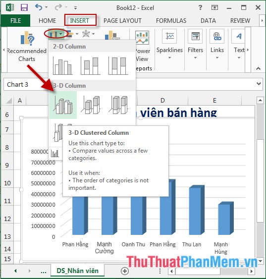
Step 2: For example, here select the type of 3D chart: Move to 3D -> click the type of chart you want to create:

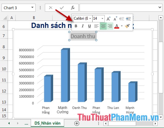
Step 3: After clicking the chart type -> chart has been created -> click on the chart name -> the Font dialog box quickly displayed, you customize it as you like:

Step 4: Click on the employee name on the chart to open the Format Axis dialog box -> change the options in the dialog box for the chart:

- Results after editing the chart:

The above is a detailed guide of steps to create charts in Excel 2013.

Good luck!