Modify the axis of the chart in Excel

The following article details you how to modify axis of a chart in Excel 2013.

As you know, the graph is made up of 2 x and y axes. The contents of the data displayed on the axes are then displayed corresponding to the axes. Modifying the axes of a chart is a modification of the description team for axial data:

To edit the contents of the axes in the chart, do the following (The example here changes the Y axis):

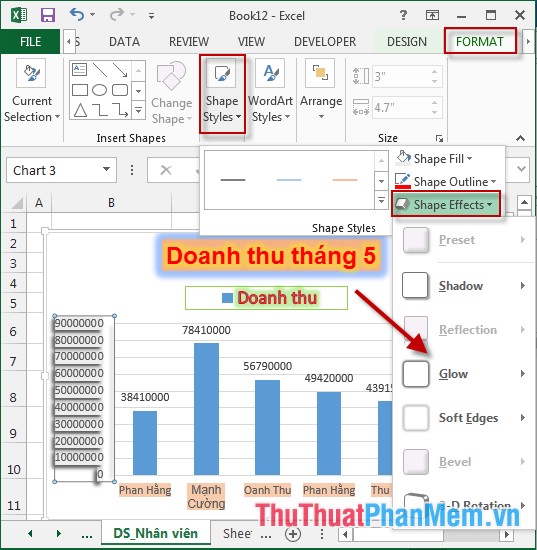
Step 1: Modify the frame of the shaft.

- Click on the axis to modify -> Format -> Shape Styles -> select properties to modify as:

+ Shape Fill: Select the fill color for the frame of the axis.

+ Shape Outline: Select a fill color for the border of the axis.

+ Shape Effect: Select the effect for the frame of the axis.

Step 2: Modify the text of the axis:

- Click on the axis to modify -> Format -> WordArt Styles-> select properties to modify as:

+ Text Fill: Select the fill color for the text content of the axis.

+ Text Outline: Select the fill color for the axis text content.

+ Text Effect: Select the effect for the text of the axis.

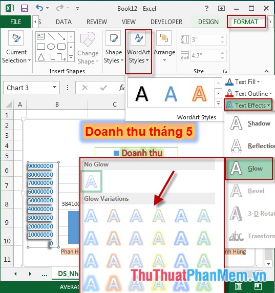
Do the same for the X axis. Notice that the content of the text displayed on the axis cannot be changed, it only changes when its content in the data table changes.

- Results after editing the content of axes:

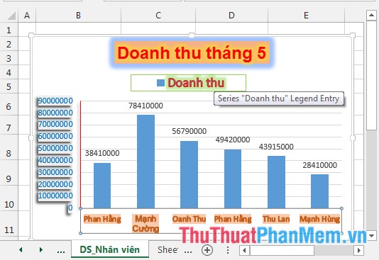
The above is a detailed guide on how to modify chart axes in Excel 2013.

Good luck!