Rotate 3D graphs in Excel

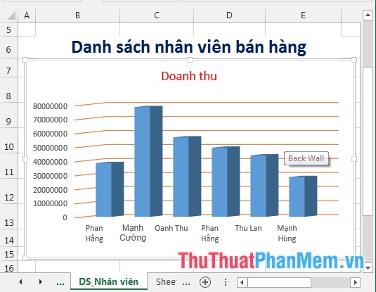
The following article details you how to rotate 3D graphs in Excel 2013.

For example, the following chart needs to be shot in 3D:

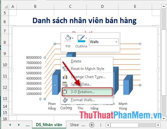
Step 1: Right-click the object in the chart -> 3-D Rotation .

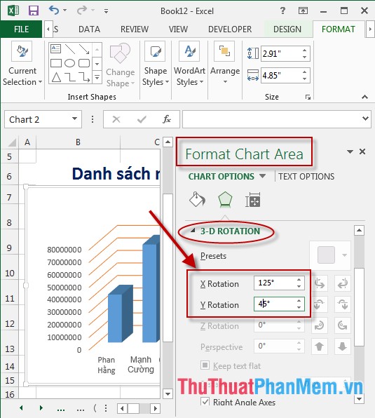
Step 2: The Format Chart Area dialog box appears -> scroll down to 3-D Rotation to enter the following data:

+ X Rotation : Enter the rotation angle for the X axis.

+ Y Rotation : Enter the rotation angle for the Y axis.

Step 3: After entering the values ​​of the graph automatically rotate according to the entered data -> results:

- Similarly, you can rotate 3-D Rotation with other objects in the chart. For example, with the content on the Y axis -> right click and choose 3-D Rotation:

- A dialog box appears that selects the rotation angle:

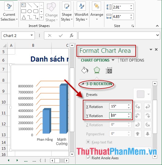
- Similarly perform 3-D Rotation with the rest of the chart objects -> get the results:

The above is a detailed guide on how to rotate 3D graphs in Excel 2013.

Good luck!