Ms Excel - Lesson 13: Use conditional formatting in Excel

Conditional formatting in Excel allows you to apply different formatting formats, such as color formatting to one or more cells based on the data of those cells.

Here are 2 simple steps to perform conditional formatting:

1. Set a condition to control formatting changes in cells

2. Enter data. If the conditions you set match the data, the format will be applied

Note : 3 conditions can be set for a cell so it can be changed to format the cell contents.

Format cells, using conditional formatting

- There are the following data, we can apply conditional formatting

Ms Excel - Lesson 13: Use conditional formatting in Excel Picture 1

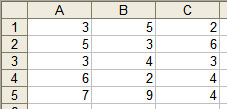
- Select the area you want to apply conditional formatting. In this example, the selected area is A1: C5 .

- From the Format menu, click Conditional Formatting .

Ms Excel - Lesson 13: Use conditional formatting in Excel Picture 2

- According to the above illustration, we will highlight all values ​​from 4 to 6, so enter the numbers into the corrected fields.

- If you click the OK button, formatting will not apply to those values. So, click the Format button

Ms Excel - Lesson 13: Use conditional formatting in Excel Picture 3

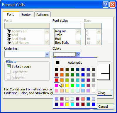
- The Format Cells dialog box displays, from which we can specify how data is displayed.

- From the Color menu : select a color, choose red for the example above.

- When done, click the OK button. The Conditional Formatting dialog box is displayed again

- To add other conditional formats, click the Add button. If not, click the OK button to skip the dialog.