How to use conditional formatting in Numbers on Mac

Conditional formatting in spreadsheets is a great feature. You only need to condition the values ​​in a cell or group of cells and when those conditions are met, the cells will be marked, formatted as text. If you want to use conditional formatting in Numbers on a Mac, read the following article.

Note: In Numbers, this feature is called Conditional highlighting.

Types of data used in conditional formatting

Before adding rules for conditional formatting, this is a list of the types of data you can use and its corresponding conditions.

1. Number : Equal, not equal, greater than, greater than or equal to, less than, less than or equal to, within and not within.
2. Text : Is, is not, begins with, ends with, contains and does not contain words or phrases.
3. Date : Yesterday, today, tomorrow, in the week / month / year, week / month / year before, week / month / next year.
4. Interval : Options are similar to numbers.
5. Blank data : empty or empty.

Set conditional formatting rules for numbers

Numbers are the most common data types used in spreadsheets such as simple numbers, money, and percentages. To set conditional formatting for numbers, we will use the product spreadsheet as an example. This data includes numbers for currency, value and inventory.

Suppose we want to quickly see when the product's inventory is below 50 by coloring these boxes in Numbers. Here's how to set it up:

Step 1 . Select the cell in the spreadsheet. You can select a group by clicking the first cell and dragging the remaining boxes or selecting the entire column or row.

Step 2 . Click the Format button on the top right to open the sidebar if you don't see it.

Step 3 . Select Cell from the top of the sidebar.

Step 4 . Click Conditional Highlighting .

Step 5 . Click Add a Rule .

Step 6 . Choose Numbers> Less than coal .

How to use conditional formatting in Numbers on Mac Picture 1

You can now customize your rules in the sidebar to apply conditional formatting. Enter the number (50) in the box according to your conditions (smaller) and then select the format from the drop-down box (red). You will see the changes immediately applied if there are values ​​that meet the conditions. Click Done .

How to use conditional formatting in Numbers on Mac Picture 2

Set conditional formatting rules for text

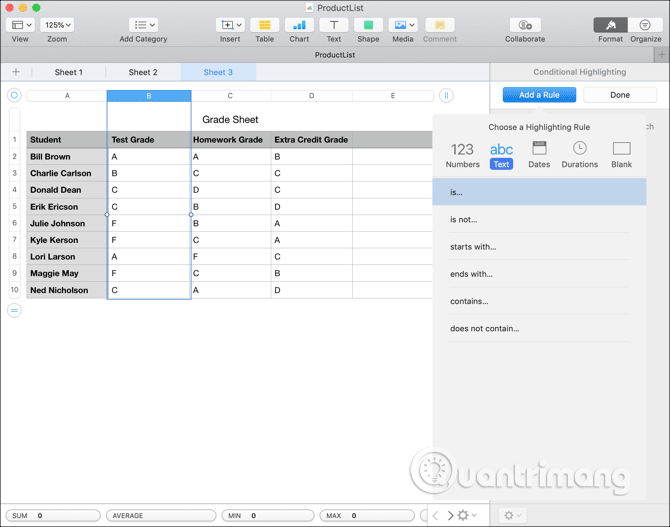
Text is also data that is used heavily in spreadsheets. This conditional formatting feature is very handy for teachers or professors who use Numbers to track student grades.

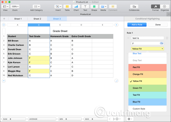
For example, in the student's transcript, we want to highlight the boxes where the students receive points F. Follow steps 1 to 5 above but this time we will choose Text and Is .

How to use conditional formatting in Numbers on Mac Picture 3

Next, customize your rules in the sidebar. Enter text (F) into the box by condition (text is) and then select your format in the drop-down box (yellow). Again, you will see immediate changes to the conditions that meet the condition. Click Done .

How to use conditional formatting in Numbers on Mac Picture 4

Set conditional formatting for dates

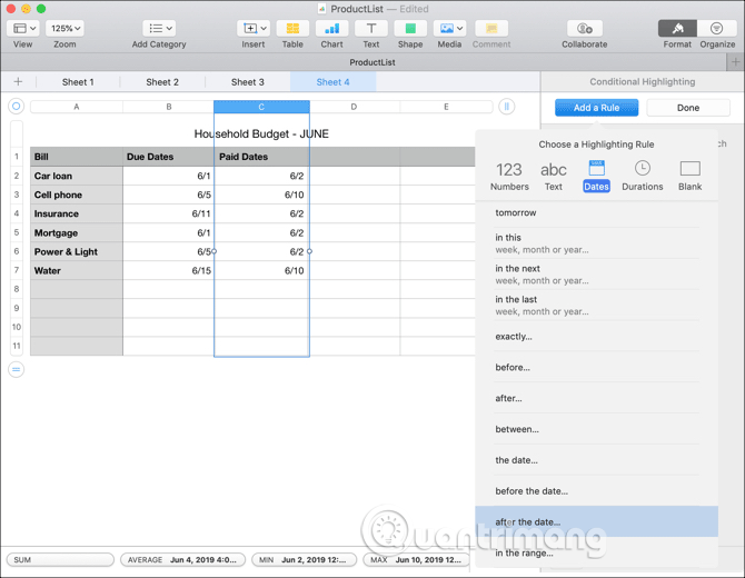
One of the best ways to use conditional formatting for the day is to highlight the billing due date. For example, we will set rules for all Paid Dates (paid dates) that have passed Due Dates (due date) showing red text.

Follow steps 1 to 5 above, then select Dates> After the date .

How to use conditional formatting in Numbers on Mac Picture 5

To easily set up this rule, instead of entering a value into the box according to conditions, like numbers or text, we will select the cells.

Click on the button inside the box you will enter the condition value. Then, select the cells that contain the date, next, click on the check mark. Now you can see that all paid dates after the due date will have red text. Click Done .

How to use conditional formatting in Numbers on Mac Picture 6

Set conditional formatting rules for time intervals

Time may not be the most popular data type in Numbers, but if you manage projects or track tasks, conditional formatting for time periods will be handy and easier to handle.

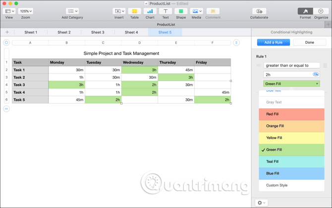
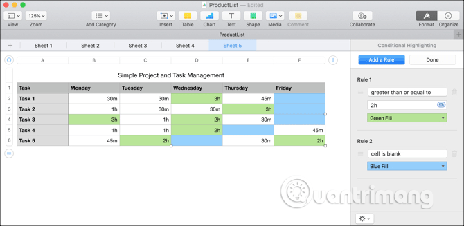
This example will use a simple project management task table. Here, we follow the time people spend on tasks each week. Now, we want to see the days when people spend two or more hours on a single task colored in green. Similarly, follow steps 1 through 5, then select Durations> Greater than or equal to .

How to use conditional formatting in Numbers on Mac Picture 7

Now, customize the rule by entering the duration (2 hours) in the box according to your conditions (greater than or equal to) and then selecting the format in the drop-down box (green). Click Done .

How to use conditional formatting in Numbers on Mac Picture 8

Set conditional formatting for empty cells

Conditional formatting for blank cells is widely used in spreadsheets to search for blank data. For example, if we have a project management worksheet, fill in the blue cells for the blank period. Follow steps 1 to 5, then select Blank> Is blank .

How to use conditional formatting in Numbers on Mac Picture 9

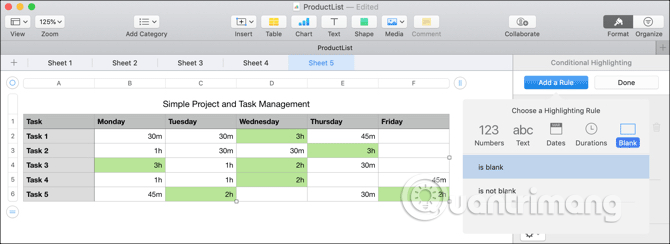
Next, simply select the color from the drop down box because there is no value under the condition, then click on Done .

How to use conditional formatting in Numbers on Mac Picture 10

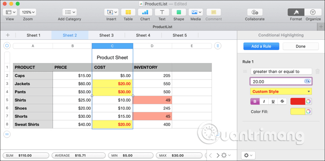
You can style yourself for the conditional formatting rules above. When it comes to selecting the format from the drop down box, go to the end and click on Custom Style . You can format the text by italics, bold, underline or dash. In addition, users can use color for text along with colored cells to combine all types of formats to suit their needs.

For example, the image below will color and highlight the letters in the box if the value of the cell is 20 USD or greater.

How to use conditional formatting in Numbers on Mac Picture 11

I wish you all success!