Use Conditional Formatting to Format Even and Odd Rows: Excel

Use Conditional Formatting to Format Even and Odd Rows: Excel covers the essential facts behind the topic, including what changed, why it mattered, and how it affected users.

Excel Overview

• To format only even rows, use the conditional formula = EVEN (ROW ()) = ROW ().
• To format only odd rows, use the following formula = ODD (ROW ()) = ROW ().

Here we will guide you through a sample example:

1. Select the rows you want to format. To select the entire worksheet, click Sheet Selector (the gray box intersects between the row and the column headers).
2. Click the Home tab.
3. Click Conditional Formatting in the Styles group and select New Rule.
4. From the Select A Rule Type list, select Use A Formula To Determine Which Cells To Format.
5. In Format Values ??Where This Formula Is True field, enter = EVEN (ROW ()) = ROW ().
6. Click Format.
7. Specify the format available. For example, to change to red for all even rows, click the Fill tab and click Red, then click OK twice.

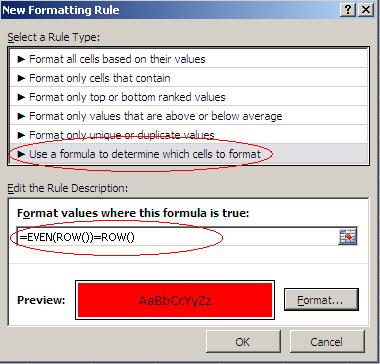
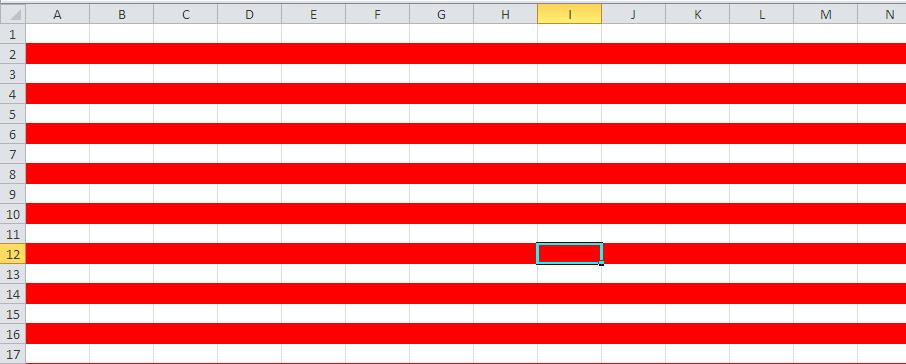
Note that all even rows are now red. To change colors for individual rows, you can repeat the steps above. In step 4, enter the formula = ODD (ROW ()) = ROW (). In step 6, select the color you like, such as blue as in our example. You should note, this technique is not only for changing colors but also for general formats.