How to create Progress bar using conditional formatting in Excel 2013, 2010 and 2007

Progress bar is very popular, it provides instant feedback on a specific process. So why not bring this convenient bar to the spreadsheet using the Conditional Formatting feature of Excel. This article will show you how to create Progress bar in Excel 2013, 2010 and 2007.

How to create the Progress bar in Excel 2013

By using conditional formatting on Excel 2013, you can create the Progress bar bar on a spreadsheet. This bar is often used to show the change of image data. Basically, you will get an effect like the chart in Excel rows and cells.

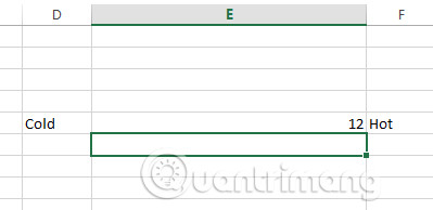
Below is an example of how to create the Progress bar. Here use data for Cold / Hot and stretch cell E to make the progress bar longer. This will help you see the bar more accurately, but this step is not required. Then enter a number in the progress box, this number will be the percentage of the selected bar.

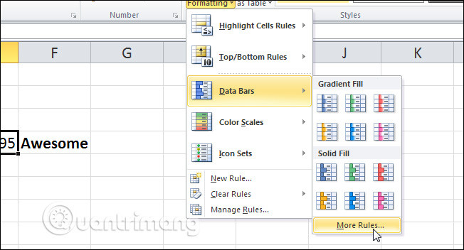
From the Excel ribbon, select Conditional Formatting and then select Data Bars> More Rules .

You should now see a window that allows you to create a new formatting rule. In this example, we adjust the settings as follows:

1. Type: select Number for both Minimum and Maximum .
2. Value : Set the Minimum to 1 and Maximum to 100.
3. Then select the color and click on OK .

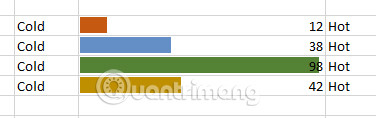
If you have adjusted all the presets correctly, you will see a progress bar as shown below.

Here is an example with many different values.

How to create the Progress bar in Excel 2010

The "Bar-type" conditional format is available from Excel 2007. But Excel 2007 only creates bars with a gradient - the bar becomes faded to the end, so even at 100%, you won't see it. It really looks like 100%. Excel 2010, 2013, solved this problem by adding a Solid Fill bar to maintain a solid color throughout.

Create a bar

The first thing you have to do is enter a numeric value in the box you want to format. You can enter values ​​directly or use formulas. For example, just enter the number in the box here.

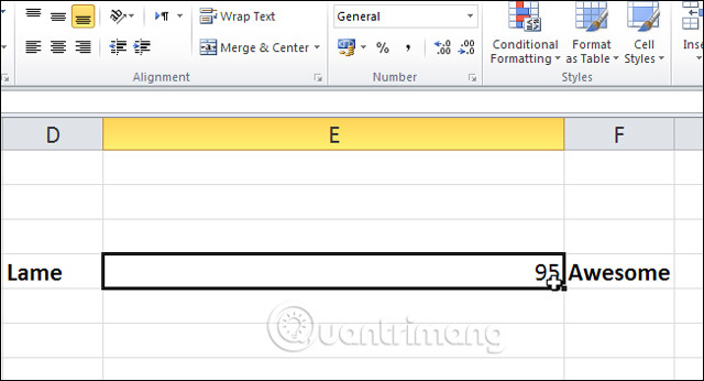
Just like above, you do not need to expand the column, but so the data will look more clear. The steps are the same as in Excel 2013, select Conditional Formatting> Data Bars> More Rules .

In the New Formatting Rule dialog box, select the Show Bar Only box (so that the number does not appear in the box). Same as above, you also set the same value.

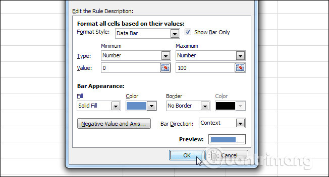
Now click on OK and you're done.

How to create Progress bar in Excel 2007

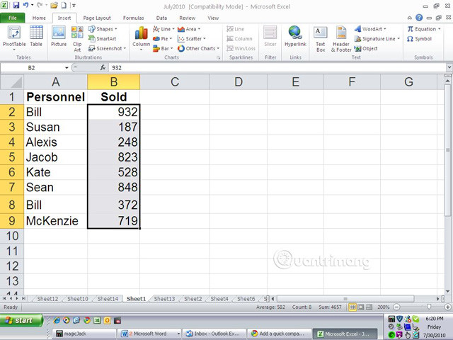
First, you will create a progress bar using conditional formatting, then make settings adjustments to adjust the size of the bar and not change the actual value that the bar represents. The following table displays a set of values ​​in column B. To display the data bar for these values, follow the steps below:

Step 1 : Choose a value from B2 to B9.

Step 2 : On the Home tab, click on the Conditional Formatting drop-down menu in the Styles group and select Data Bars.

Step 3: Choose an option from galley .

As a result you will see a series of comparison bars for each value. Each bar will represent the relationship with the other bars. For example, the highest value in cell B2, takes up nearly the entire cell, while the lowest value B3 is only about 20% of the value for cell B2 and accounts for about one fifth of the cell.

Now change the rules a bit but still perform on the same data for easy comparison.

After creating the data bar, select Manage Rules from the Conditional Formatting drop-down menu. In the resulting dialog box, click Edit Rules . The default rule is Format All Cells Based On Their Values and we need to change this rule. In the Edit Rule Description section , set the Minimum and Maximum values ​​to Automatic . Change the Minimum Type to Number and Excel will set the Value to 0, then click OK twice.

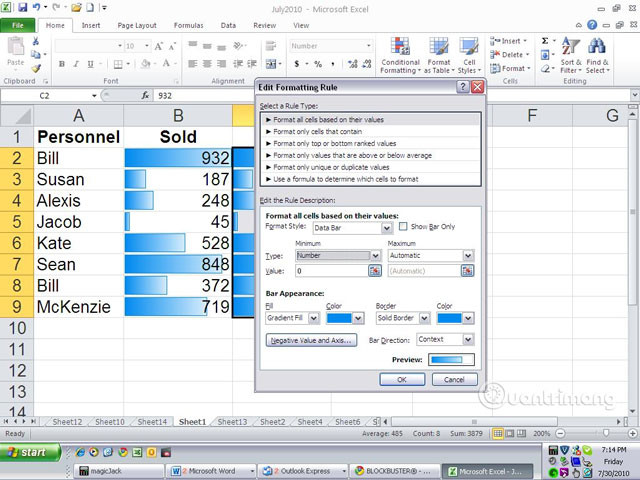
Not much change for higher values. However, the lowest value bar has disappeared completely. In addition, the bars for the lower numbers will be smaller. That's because above we have changed the ratio between the set of values ​​by reducing the lower value to 0.

Now try changing the other rules. This time, select Number from the Type drop-down list for both Minimum and Maximum values. In Minimum Value , enter 0; Enter 1000 for the Maximum value.

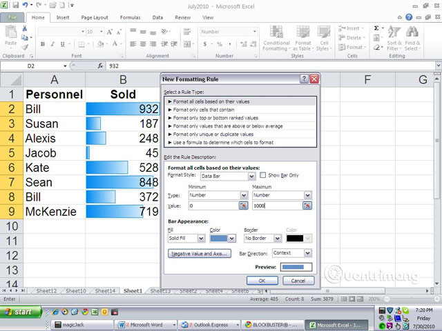
This time, all the bars seem to only adjust slightly, but the most significant change is in the highest value bar. As you can see, it no longer takes up nearly all of the cells, because the bars represent values ​​between 1 and 1000.

See more:

1. How to format conditional cells in Google Sheets
2. Use conditional formatting to format even and odd rows
3. 8 convenient tools in Excel you may not know yet