How to use Conditional Formatting to conditional formatting in Excel

How to use Conditional Formatting to conditional formatting in Excel Picture 1

Excel has a Condititional Formatting tool that is quite adequate for the needs of users. However, the built-in formats of Excel are not enough to meet your needs, Excel supports users to easily create new rules.

The format rules are available in Conditional Formatting

Conditional Formatting is located in the Home tab. To set the format for a range / column / row of data, select (highlight) the data range. Select the Home tab (1) and click on the Conditional Formatting icon (2) .

How to use Conditional Formatting to conditional formatting in Excel Picture 2

Highlight cells Rules - Rules highlight cell colors according to value rules

1. Greater than: Greater value.
2. Less than: Prices are smaller.
3. Between: Value in the range.
4. Equal to: Value is equal to.
5. Text that Contains: The value contains a string of characters.
6. A Date Occciring: The value contains a predefined date.
7. Duplicate Value: Duplicate value.

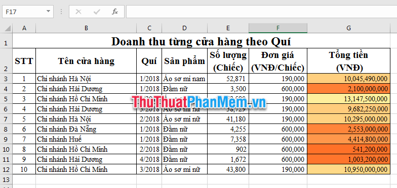
For example, in the table above, you find the revenue values ​​greater than 4,000,000,000 and highlight that cell color => You select Greater than. In the value comparison section, you type the number 4,000,000,000,000 (1) . In the highlighted color section (2) , you can choose from the available Excel formats or customize by selecting Custom Format .

How to use Conditional Formatting to conditional formatting in Excel Picture 3

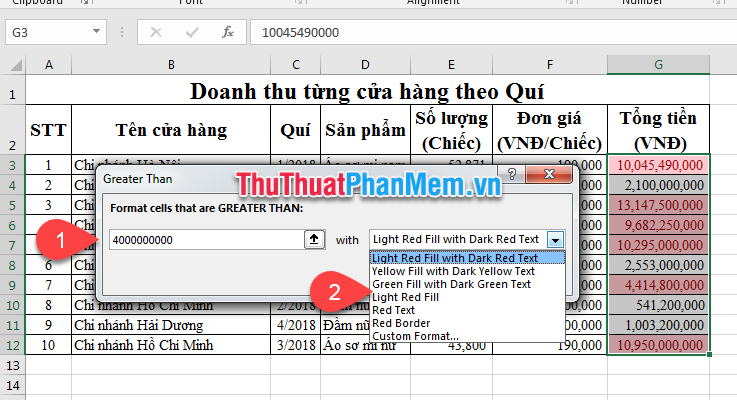
After selecting all the options, click the OK button. As a result, cells containing values ​​greater than 4,000,000 are highlighted.

Top / Botton Rules - The rules for determining cells by rank

Excel determines the cell's rank in the data range and formats that cell.

How to use Conditional Formatting to conditional formatting in Excel Picture 4

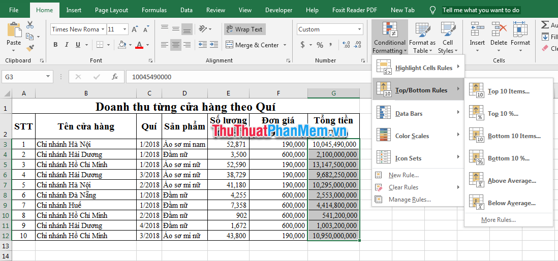
1. Top 10 Items: Format the 10 cells with the largest value.
2. Top 10%: Format 10% of the maximum number of cells.
3. Bottom 10 Items: The 10-cell format with the lowest value.
4. Bottom 10%: Format 10% of the minimum number of cells.
5. Above Average: Format cells that are larger than the average of the data range.
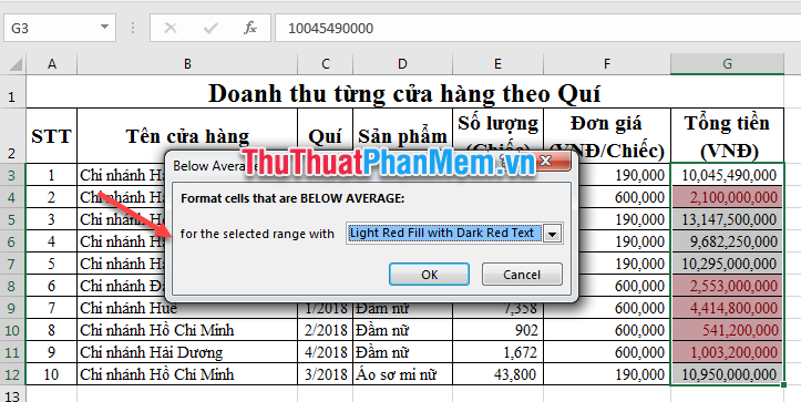
6. Below Average: Format a cell smaller than the average value of the data range.

For example, the table above, you need to format the color cells smaller than the average value of the data range, select Below Average. The format options window appears, you can choose the available formats of Excel or customize by selecting Custom Format . Then press the OK button .

How to use Conditional Formatting to conditional formatting in Excel Picture 5

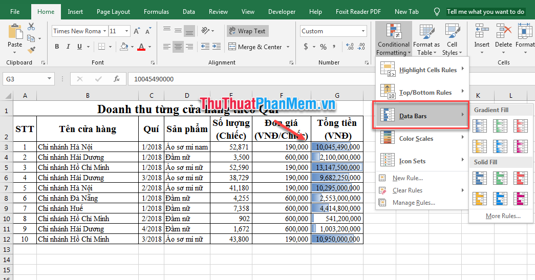
Data Bar - Format the size of each value

With this format, the size of each cell in the data range will be determined by long or short highlighting.

How to use Conditional Formatting to conditional formatting in Excel Picture 6

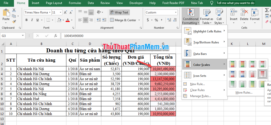
Color Scale - A rule to organize data in ascending and descending order according to the color density

This rule will arrange the order of each cell in the string and highlight the color according to the format that the user chooses.

How to use Conditional Formatting to conditional formatting in Excel Picture 7

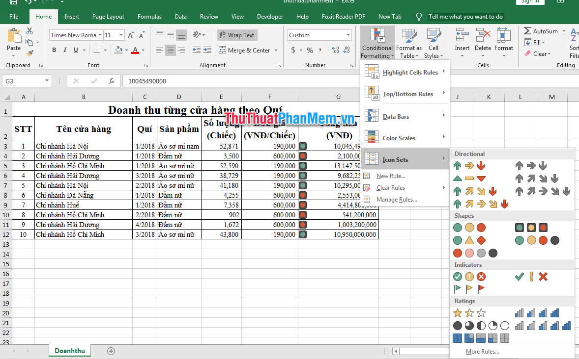
Icon Set - Add symbols in the value box

With this type of format, Excel groups data by special symbols such as arrows, traffic lights, etc.

How to use Conditional Formatting to conditional formatting in Excel Picture 8

Create a new format rule in Excel

If the types of formatting rules available do not meet the needs of the report, you can set up the new format by:

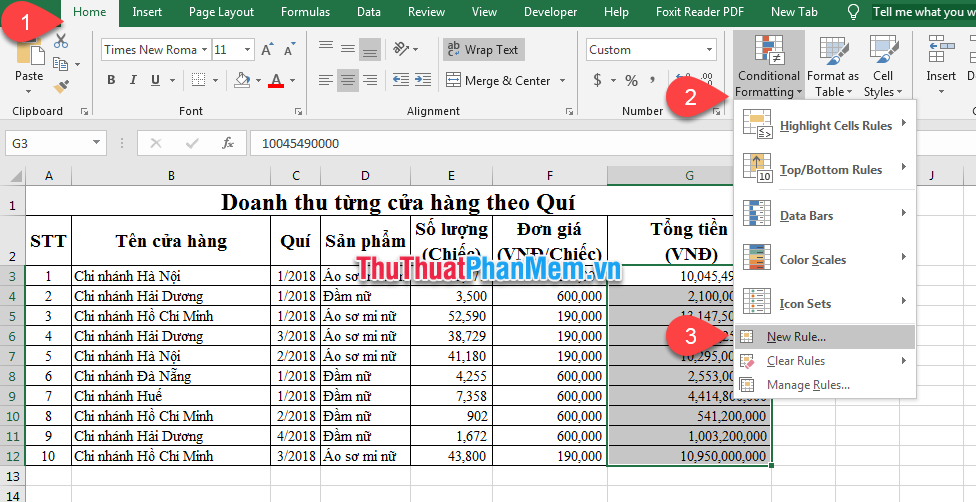
Step 1: Select (black out) the data area to be changed. On the Home tab (1 ), click on the Conditional Formatting icon (2) and select New Rule (3) .

How to use Conditional Formatting to conditional formatting in Excel Picture 9

Step 2: New Formatting Rule window appears.

How to use Conditional Formatting to conditional formatting in Excel Picture 10

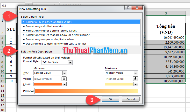
(1) Select a Rule Type : select the type of data classification you need to perform.

1. Format all cells based on their values: Apply background color to all cells based on the value of the data range.
2. Format only cells that contain: Apply cell background color that contains a certain data.
3. Format only top or bottom ranked values: Highlight the first or last ranking cells in the selected data range.
4. Format only values ​​that are above or below average: Highlight the cells with values ​​above or below the average value.
5. Format only unique or duplicate values: Highlight cells with unique values ​​or duplicates in the selected data range.
6. Use a formula to determine which cells to format: Use another formula to color.

(2) Edit the Rule Description : Optionally set the description for the data classification type you selected above.

With the above settings, Dexterity Software has set the format for the largest number, the color is orange and darker to the smallest. The results are as follows:

How to use Conditional Formatting to conditional formatting in Excel Picture 11

Delete and manage formatting rules

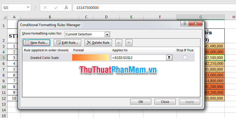
To check and manage format rules, go to Conditional Formatting and select Manage Rules. The Manage window will appear, based on this window you can know which cell rules are applying. Here you can add formatting, edit / edit formats and delete formatting.

How to use Conditional Formatting to conditional formatting in Excel Picture 12

To delete all Conditional Formatting formats , you cannot edit by Fill (highlight the cell color), but you must delete the installed format by:

Step 1: You only black out the data area but need to delete the format. On the Home tab (1 ), click on the Conditional Formatting icon (2) and select Clear Rules (3) .

In which: Clear rules from selected Cells is to delete the format in the currently selected cell.

Clear rules from entire Sheet is to delete all formatting from the open worksheet.

Above Software Tips showed you how to use Conditional Formatting format tool in Excel. Good luck!.