3 ways to highlight cells or rows in Excel

Microsoft Excel comes with a number of features that allow users to create spreadsheets from basic to advanced, making professional life easier. However, when dealing with large, complex data sets in Excel, it is easy to lose interest.

One easy way to simplify your spreadsheet is to highlight checkboxes and rows with checkboxes so that they stand out. The following article will discuss in detail different ways to do this.

Highlight cells or rows using VBA code

To highlight a cell or row in Excel that has a checkbox, the first method we will discuss involves using VBA code. VBA is basically a programming language in Excel that is used to automate tasks. You enter the code relevant to your requirement and Excel will do the task for you, saving you hours of manual work.

We all know that it takes hours in Excel when you have to do everything manually. VBA code handles large amounts of data to make this process easier for you. Follow these steps to proceed with this method:

1. Launch Excel and open the targeted worksheet.

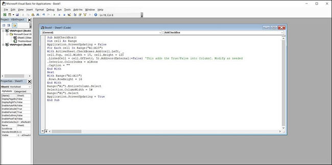
2. Right-click on the Sheet tab at the bottom and select View Code from the context menu.

3. This will open the Microsoft Visual Basic for Applications dialog box . Copy the code mentioned below and paste it in the VBA window. You can modify the cell range, height and width as per your requirement.

Sub AddCheckBox()Dim cell As Range Application.ScreenUpdating = False For Each cell In Range("A1:A12") With ActiveSheet.CheckBoxes.Add(cell.Left, _ cell.Top, cell.Width = 17, cell.Height = 15) .LinkedCell = cell.Offset(, 5).Address(External:=False).Interior.ColorIndex = xlNone .Caption = "" End With Next With Range("A1:A12") .Rows.RowHeight = 17 End With Range("A1").EntireColumn.Select Selection.ColumnWidth = 6# Range("B1").Select Application.ScreenUpdating = True End Sub

Highlight cells or rows using Conditional Formatting

The next method on the list to highlight a cell or row is to use the Conditional Formatting option. Conditional Formatting allows users to modify the appearance of cells based on preferred criteria.

In this method, the article will apply a condition that will label the highlighted checkboxes as True and highlight them (this can be modified as per your requirement). The rest of the rows will be in a standard format, making it easy to differentiate between completed and incomplete tasks.

Here's how you can use Conditional Formatting to highlight a cell or row:

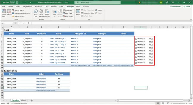
1. Before you can apply conditional formatting, you must add check boxes to your table. To do this, go to the Developer tab in Excel.

2. In the Controls section , select Insert and click the check box icon in the Form Controls section.

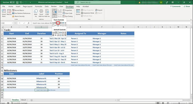
3. Add checkboxes to the cells you want.

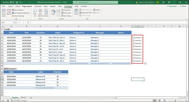
4. Then, select the cell with the checkbox and drag the cursor to the bottom of the table. This will add the checkbox to all cells in the table.

5. Now, right-click on the first cell with the checkbox and select Format Control from the context menu. This will launch the Format Object dialog box.

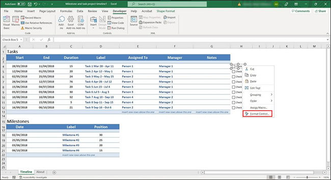
6. Find the Cell link option and enter the name of the cell you want to link your first checkbox to. For example, our first checkbox is in cell H4 and we want to label the cell right before it, so we'll add I4 to the text field.

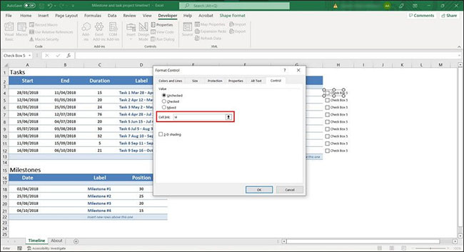
7. Click OK to apply the changes and perform the same steps for the rest of the check boxes in the table.

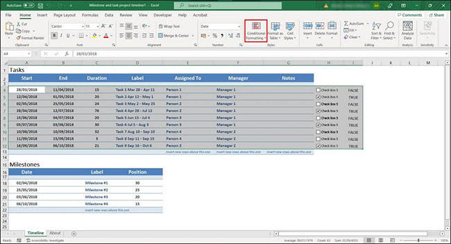
8. Once done, select the rows you want to highlight and click on the Conditional Formatting option in the Home tab.

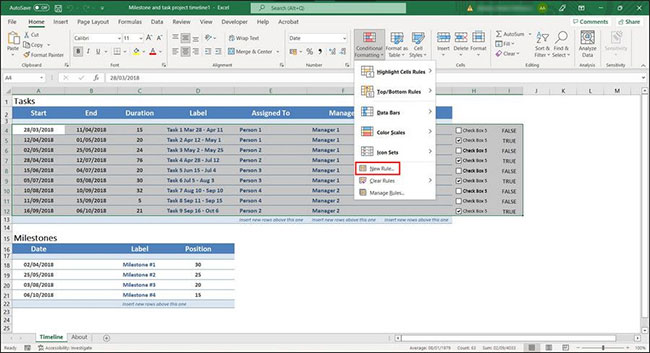
9. Select New Rule from the context menu.

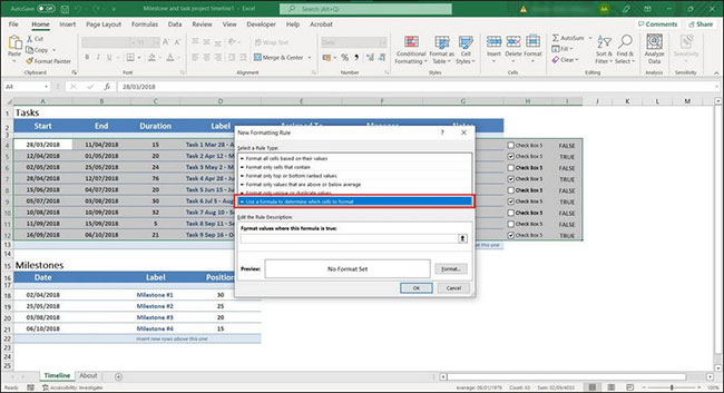
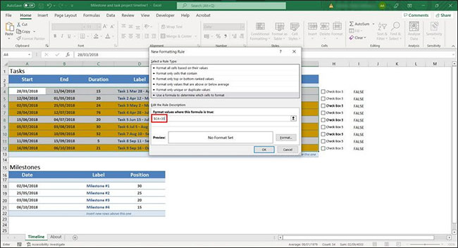
10. In the following dialog box, click Use a formula to determine which cells to format in the Select a Rule Type option .

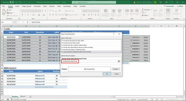
11. Now go to Edit the Rule Description section and enter =IF($I4=TRUE,TRUE,FALSE) in the text field.

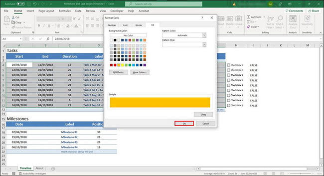
12. Click the Format button and choose a highlight color.

13. Then click OK to save the changes.

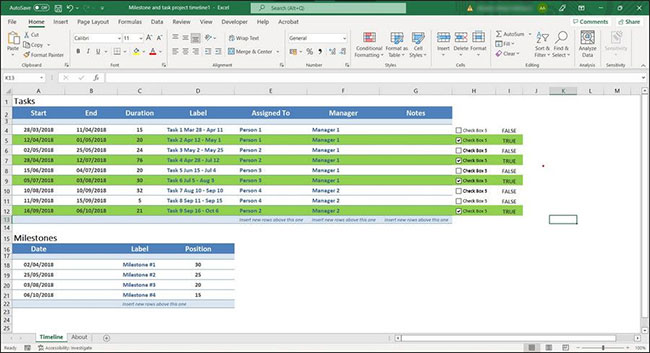
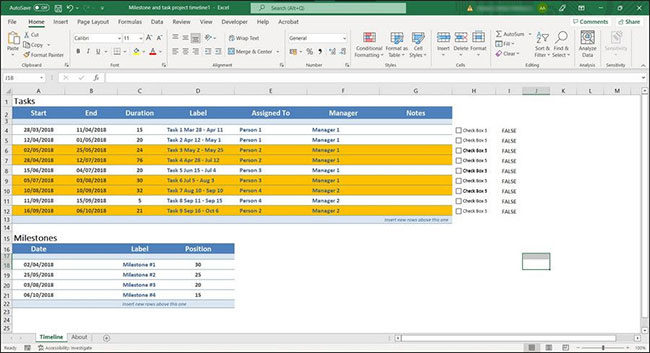
The selected rows or cells will be highlighted with conditional formatting.

Highlight rows with different colors using Conditional Formatting

Sometimes you want to highlight different rows with different colors to better organize your spreadsheet. Luckily, Conditional Formatting allows you to do that too.

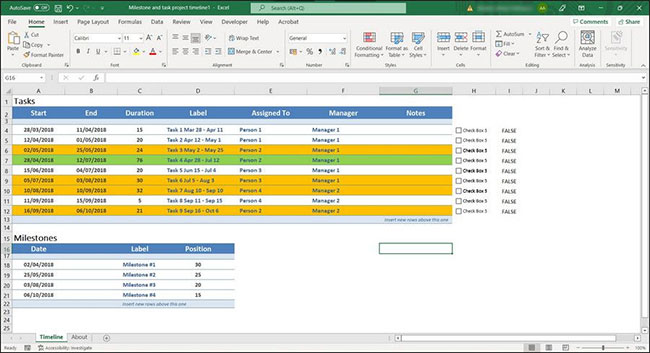
For example, if you are listing your to-dos and want to highlight items that are due more than 30 and 45 days in duration, you can highlight such items in different colors. Here's how:

1. Select the rows in the table that you want to highlight (usually the entire data set).

2. In the Home tab and click the Conditional Formatting option.

3. Select New Rules.

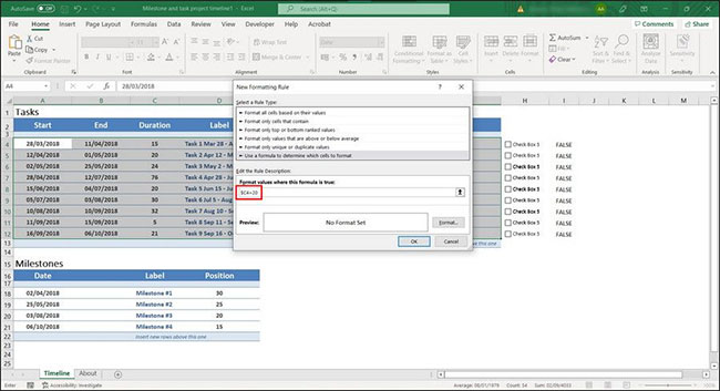
4. In the following dialog box, select Use a formula to determine which cells to format in the Select a Rule Type section .

5. Enter the following formula in the text field for Format values ​​where this formula is true . Remember that the article is applying the formula according to the example table. To make this method work in your case, you will have to change the values ​​accordingly.

$C4>20

6. Click the Format button and choose a color.

7. Click OK to save the changes.

8. Finally, click OK again. Items older than 20 days will be highlighted.

9. Now, select the New Rule button again and click Use a formula to determine which cells to format under Select a Rule Type .

10. Enter the following formula in the Format values ​​where this formula is true text field .

$C4>35

11. Click the Format button and choose a color.

12. Select OK.

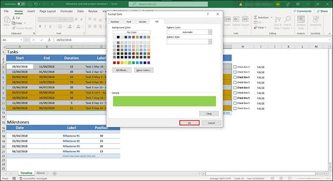
13. Click OK again to save the changes.

This will help you highlight rows and cells with different colors in Excel. If you want to cross something out in your spreadsheet, you can strikethrough it in Excel.

Highlighting rows and cells in an Excel spreadsheet can have many benefits. In addition to bringing your spreadsheet to life, doing so makes your data easier to see.

David Pac

Update 12 January 2025