How to use conditional formatting in Microsoft Excel 2016

Introduce

Conditional Formatting is a powerful tool and can change the 'appearance' of a cell based on its value, helping viewers to identify important data quickly. You can add colors, icons, data bars and color scales to the cell by creating conditional formatting rules.

Mark duplicate values ​​in red

Conditional formatting can be used to highlight duplicate values, making it easy to identify and correct errors in data.

How to use conditional formatting in Microsoft Excel 2016 Picture 1

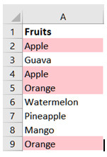
Steps to take:

Step 1 . Select the cells to format. In this example are cells A2: A9.

Step 2 . Go to Home> Conditional Formatting .

Step 3 .Click on Highlight Cells Rules> Duplicate Values .

How to use conditional formatting in Microsoft Excel 2016 Picture 2

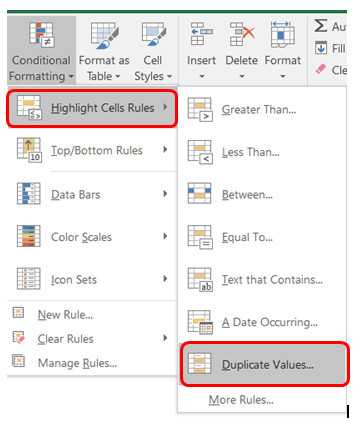
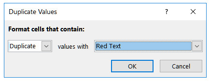
Step 4 . Click OK . You can also select other cell colors from the drop-down list next to the default list.

How to use conditional formatting in Microsoft Excel 2016 Picture 3

Use Data Bars to create Progress Bars (progress bar)

Data Bars can be used to display data graphically within a cell. The longest bar represents the highest value and the shortest bar shows the smallest value. This Data Bars help users to find large and small quantities easily in spreadsheets.

In this example, you will quickly see the progress of the projects.

How to use conditional formatting in Microsoft Excel 2016 Picture 4

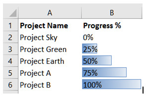
Steps to take:

Step 1 . Select the cells to format. In this example, B2: B6.

Step 2 . Go to Home> Conditional Formatting.

Step 3 . Click Data Bars> Blue Data Bar .

How to use conditional formatting in Microsoft Excel 2016 Picture 5

Step 4 . You can also choose other color bars if you want.

See also: How to create Progress bar by conditional formatting in Excel 2013, 2010 and 2007

Use the Top / Bottom Rules rules to highlight the top 3 products

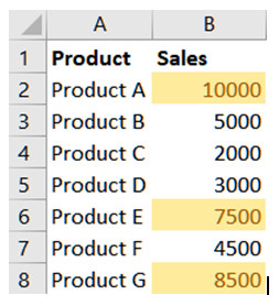
Another great way to use conditional formatting is to select the Top / Bottom Rules option. You can easily mark the top 3 items in the list. To determine the top three products that generate the most sales in the store, you can create a top rule in conditional formatting.

How to use conditional formatting in Microsoft Excel 2016 Picture 6

Steps to take:

Step 1. Select the cells to format. In this example, B2: B8.

Step 2 . Go to Home> Conditional Formatting .

Step 3 . Click on Top / Bottom Rules> Top 10 Items .

How to use conditional formatting in Microsoft Excel 2016 Picture 7

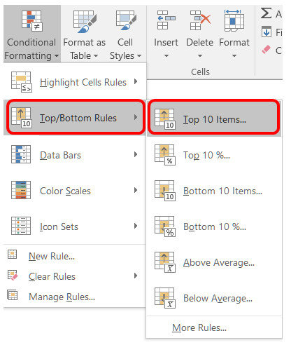
Step 4. The default is 10 items but you can enter 3 or use the add or remove buttons.

How to use conditional formatting in Microsoft Excel 2016 Picture 8

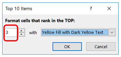
Step 5 . You can also select other cell colors from the drop-down list next to the default list.

Using Color Scales to create a heat map

What is heat map?

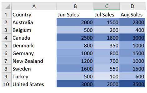
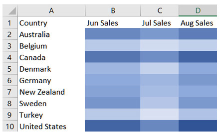
Heat map is a table in which spreadsheet data is displayed in color. You can display the value in the box or not if you want. Hide the value using the cell format.

How to use conditional formatting in Microsoft Excel 2016 Picture 9

Steps to take:

Step 1 . Select the cells to format. In this example, B2: D10.

Step 2 . Go to Home> Conditional Formatting.

Step 3. Click on Color Scales> More Rules .

How to use conditional formatting in Microsoft Excel 2016 Picture 10

Step 4 . The default is 2-Color Scale, but you can select 3-Color Scale from the drop-down list.

How to use conditional formatting in Microsoft Excel 2016 Picture 11

Step 5. For this example, light blue, blue and dark blue are selected. When choosing a color for a heat map, you should choose different colors for the same color. Because if you choose different colors will confuse viewers, it is difficult to determine which cells have the lowest or highest value. However, when choosing different colors for the same color, viewers can quickly recognize the highest and lowest values.

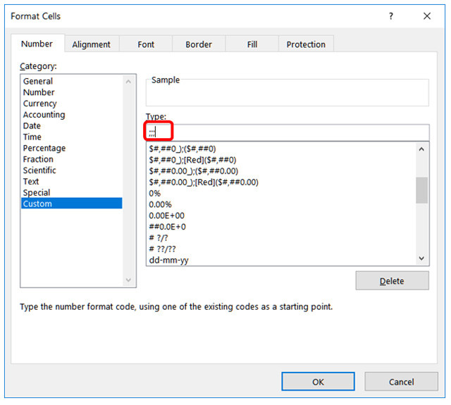
Also, if you want to hide the values ​​in the table and display only the color in the heat map, you can right-click on the worksheet, click Format cells> Custom> Enter ';;;' in the box type and click on OK . The value is still in the table but hidden.

How to use conditional formatting in Microsoft Excel 2016 Picture 12

Heat map after hiding value:

How to use conditional formatting in Microsoft Excel 2016 Picture 13

Use Icon Sets to identify missing data in Timesheet

Many opinions suggest that conditional formatting can only be used to format cells based on its value. However, you can use the formula to get values ​​based on cells in the same row and then use conditional formatting to get the desired results.

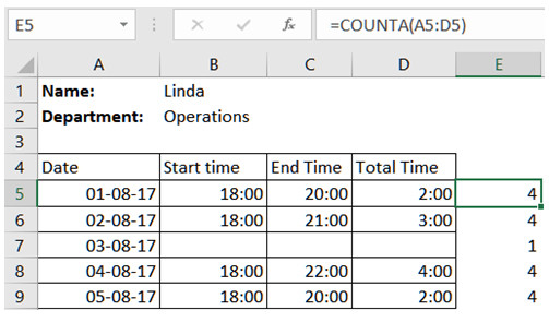
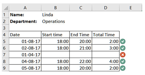
See this example for a better understanding. In this example, we will execute the formula in cell E4 to calculate the number of cells that have been filled in from A5 to D5. Since all the necessary data has been filled in row 5, the formula displays the results of the 4 cells that have been populated. However, in row 7, there is only 1 cell with data and 3 empty cells. Therefore, this row needs to be highlighted using Icon Sets to determine the row to be adjusted.

How to use conditional formatting in Microsoft Excel 2016 Picture 14

Steps to take:

Step 1 . Select the cells to format. In this example is E5: E9.

Step 2 . Go to Home> Conditional Formatting .

Step 3 . Click on Icon Sets> More Rules .

How to use conditional formatting in Microsoft Excel 2016 Picture 15

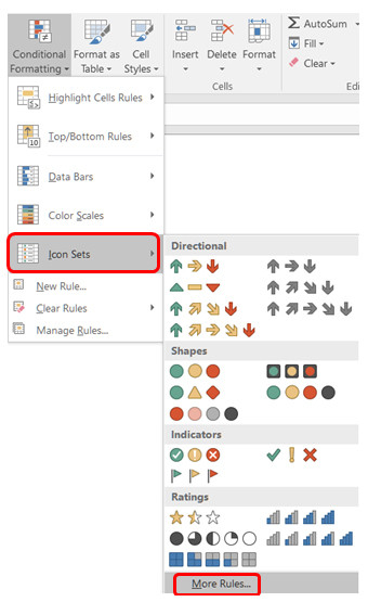
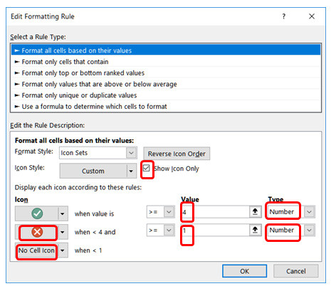
Step 4 . The default option here is 3 traffic lights, then select 3 icons (circle) from the drop-down list.

Step 5. Check the ' Show Icon only ' box.

Step 6 . Click on the last icon and change ' Red Cross Symbol ' to ' No Cell Icon '.

Step 7. Click on the second icon, change the ' Yellow Exclamation Symbol ' to ' Red Cross Symbol ', change the value to 1 and change the Type from ' Percent ' to ' Number '.

Step 8 . For the first symbol is ' Green Check Symbol ', change the value to 4 and change the Type from ' Percent ' to ' Number '.

How to use conditional formatting in Microsoft Excel 2016 Picture 16

After completing the above steps, if there are unfinished data in any cell in the AD column of the same row, there will be a slash in column E. This will allow the user to quickly identify the data. Incomplete material and repair it. When all four cells from the AD column are entered in the same row, a green check mark will appear. This will allow the user to know that all data has been entered and no data is missing.

How to use conditional formatting in Microsoft Excel 2016 Picture 17

Delete rule

Define cells that contain conditional formatting

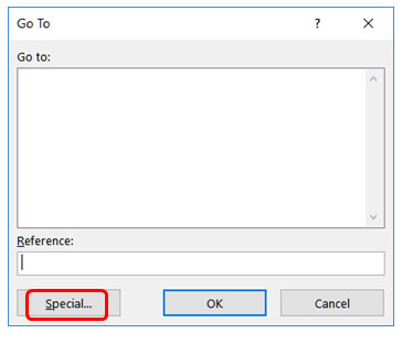
Before deleting all conditional formatting, you need to specify a cell containing conditional formatting. To do this, select all cells on the spreadsheet using Ctrl + A , click Special> Conditional formats> OK .

How to use conditional formatting in Microsoft Excel 2016 Picture 18

How to use conditional formatting in Microsoft Excel 2016 Picture 19

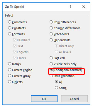
This will show you the cells marked with E5 to E9 contain conditional formatting.

How to use conditional formatting in Microsoft Excel 2016 Picture 20

Delete the cell containing conditional formatting

Steps to take:

Step 1 . Go to Home> Conditional Formatting .

Step 2. Click Clear Rules> Clear Rules from Selected Cells .

How to use conditional formatting in Microsoft Excel 2016 Picture 21

Delete multiple rules in the same sheet

In addition, there is another way to delete conditional formatting. This method will show all cells using conditional formatting on the same worksheet and allow you to delete multiple rules easily.

Steps to take:

Step 1 . Go to Home> Conditional Formatting.

Step 2 . Click on Manage Rules .

How to use conditional formatting in Microsoft Excel 2016 Picture 22

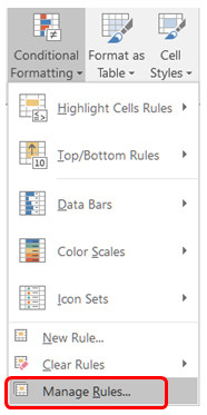
Step 3 . Change the rule Show formatting from Current Selection to This Worksheet. This will display all the rules in this spreadsheet.

Step 4 . Click on the rule you want to delete → click on Delete Rule → OK.

How to use conditional formatting in Microsoft Excel 2016 Picture 23

Step 5 . Repeat Step 4 for the rules you want to delete.

I wish you all success!

See more:

1. Use conditional formatting to format even and odd rows
2. Complete guide to Excel 2016 (Part 1): Get familiar with Microsoft Excel
3. 5 nightmares for Excel and how to fix it