Instructions on how to create flashing text in Excel

If you want to highlight text in your Excel spreadsheet, creating flashing text is a cool trick. The tutorial below will help you do it quickly, with detailed and easy-to-understand steps.

How to create flashing text in Excel

Step 1: Open your Excel file. Here, press Alt + F11 to open Excel's VBA code interface .

Step 2: The Microsoft Visual Basic for Applications dialog box appears. Click on the Insert menu -> then select Module as shown below.

Then Copy the Code below:

Sub StartBlink()
Dim xCell As Range
Dim xTime As Variant
Set xCell = Range("A1")
With ThisWorkbook.Worksheets("Sheet1").Range("A1").Font
If xCell.Font.Color = vbRed Then
xCell.Font.Color = vbBlue
Else
xCell.Font.Color = vbRed
End If
End With
xTime = Now + TimeSerial(0, 0, 1)
Application.OnTime xTim, "'" & ThisWorkbook.Name & "'!StartBlink", , True
End Sub

Next, you paste it into the Module window . Then press Alt + Q to close the dialog box.

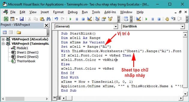
Note: In the above code, you need to replace the cell position where you entered the text you want to flash and which Sheet you are working on, please edit it correctly.

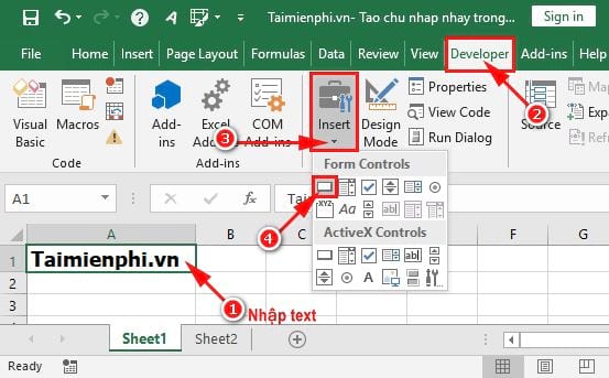
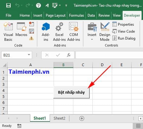
Step 3: Enter the text into the cell where you want it to flash -> then click to open the Developer tab -> select Insert and Button (Form control).

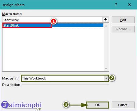
Step 4: Then, drag the mouse to create a Button on the Excel file. At this time, the Assign Macro dialog box will appear. In the section:

- Macro name: You choose StartBlink

- Macros in: You set it to This Worknook

This action is intended to flash only the text in the current Sheet. Then you press OK to create the Button .

Step 5: Next, right-click on Button -> and select Edit Text .

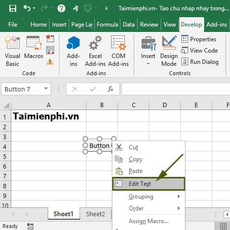
You can then rename the Button to whatever name you want and click to enable flashing mode.

So, you have learned how to create flashing text in Excel using VBA code to highlight important information. Applying this trick will help easily draw attention to data cells that need to be emphasized.

In addition, if you want to optimize your spreadsheet, you can refer to the method of  alternating colors in Excel  to distinguish data without having to do it manually. This is a very useful method to save time and increase the visualization of the spreadsheet.

Jessica Tanner

Update 19 February 2025