How to use Style in Excel

With MS Excel data often has the same format in the same group. Therefore, to save time and ensure consistency in data format helps readers have a better overview of the following article on how to use Style in Excel.

1. Apply the Style formats available in Excel.

For example, you need to format the table header.

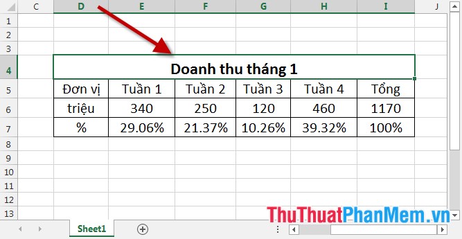
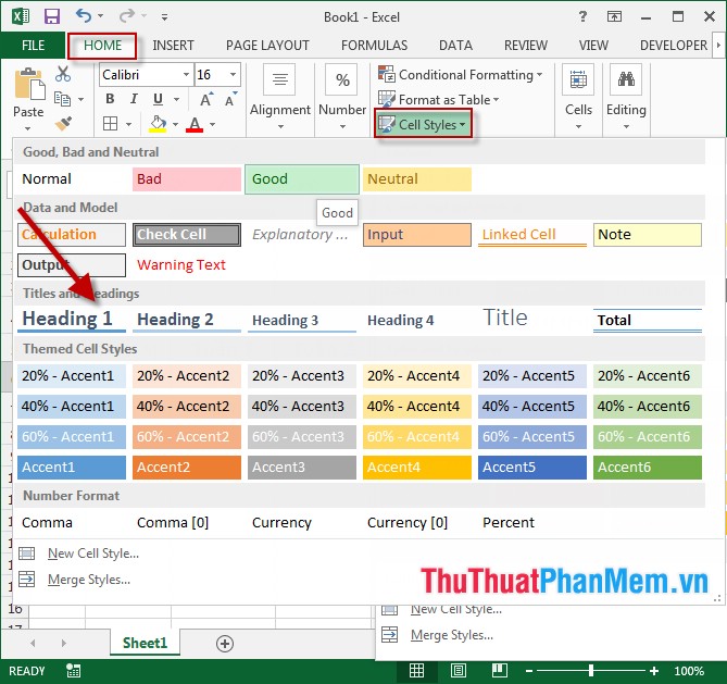
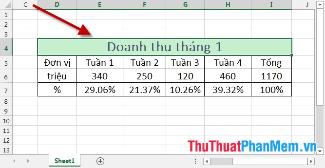
Click on the cell you want to format -> Home -> Cell Styles -> choose the format you want:

2. Create your own style as you like.

Step 1: Go to the Home tab -> Cell Styles -> New Cell Style . to create your own Style :

Step 2: The Style dialog box appears and gives the Style name in Style Name -> check  the box for numbers, margins, fonts, borders and colors. In addition, to select other formats, click Format:

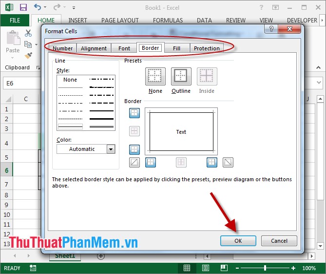
Step 3: The Format Cells dialog box appears, select the cards corresponding to the formats -> finally click OK:

Step 4: Finally, click OK to close the Style dialog box :

Step 5: Go back to the Excel file -> Home -> Cell Styles -> select the Style corresponding to the Style just created, the example here is Excel_Fast:

Results after selecting your own custom Style :

Above is a detailed guide on how to use Style in Excel. Good luck!