How to filter duplicate data on 2 Excel sheets

In basic Excel functions, Vlookup function is also used frequently. Vlookup function belongs to the function of searching data on Excel and we can combine functions with many other functions to process data, such as Vlookup function with If function, Vlookup function with Left function, using Vlookup function to combine 2 tables, .

In this article, Network Administrator will introduce how to use Vlookup function to filter duplicate data from 2 different sheets. Filtering duplicate data on Excel in a single sheet is relatively simple, just use the available filtering feature. But if 2 or more sheets, users can use Vlookup function.

1. How to automatically display names when entering code in Excel
2. How to combine Sumif and Vlookup functions in Excel
3. How to use AVERAGEIF function in Excel

1. Use Vlookup function to filter Excel duplicate data

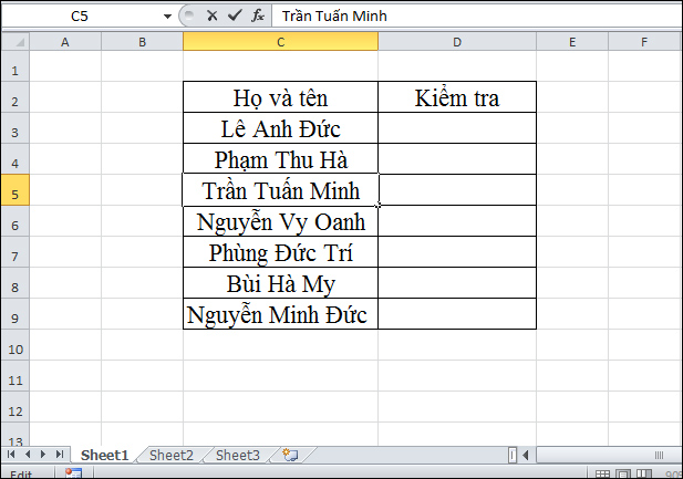
We will have 2 data tables below. In Sheet 1 will be the name column to filter duplicate data and Sheet 2 is the main data.

How to filter duplicate data on 2 Excel sheets Picture 1

Sheet 2 has the data sheet as shown below.

How to filter duplicate data on 2 Excel sheets Picture 2

Step 1:

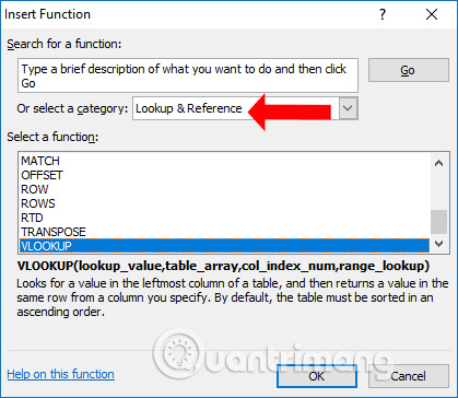
In Sheet 1 in the first cell enter the same result, click on the Formulas tab and select Insert Function .

How to filter duplicate data on 2 Excel sheets Picture 3

Step 2:

The Insert Function dialog box appears. In the Or select a category section, you will find the Lookup & Reference group because Vlookup function belongs to the search function group.

Scroll down to the bottom of the list and see the VLOOKUP function , click OK.

How to filter duplicate data on 2 Excel sheets Picture 4

Step 3:

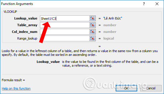
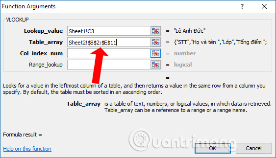
Next to display the Function Arguments dialog box. Here the user will enter data areas for each element.Lookup_value section, click on Sheet 1 and then click on cell C3 . Box C3 is the first box containing the name in Sheet 1.

Then the Lookup_value box will appear Sheet1! C3 .

How to filter duplicate data on 2 Excel sheets Picture 5

At Table_array click on Sheet 2 and select the entire area of ​​the data to be checked for the same. At Table_array, Sheet2 will appear ! C2: E11 with C2: E11 is the data area.

How to filter duplicate data on 2 Excel sheets Picture 6

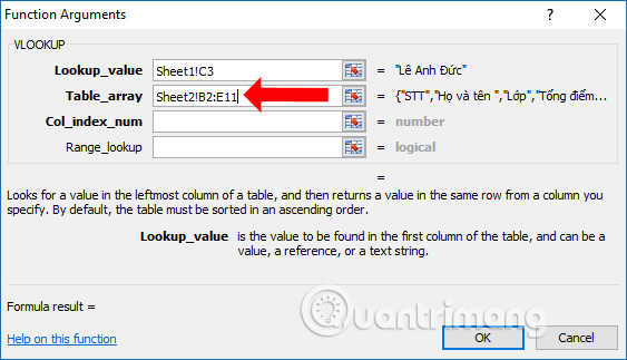
Readers need to note that if they want to check a lot of data, they need to fix the selection by clicking on the middle or the end of C2 and pressing F4, similar to E11 to be fixed. Now Table_array will be Sheet2! $ C $ 2: $ E $ 11 as shown below.

How to filter duplicate data on 2 Excel sheets Picture 7

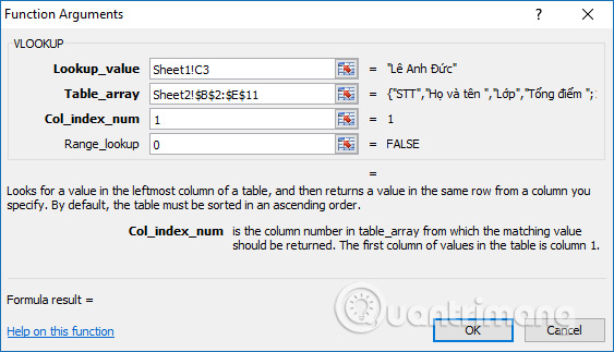
In Col_index_num, enter the position of the column you want to return data if it is the same. For example, the column of data that you want to check will be in the first column, so enter 1.

Range_lookup you enter 0 for the search function to be exact. Finally click OK.

How to filter duplicate data on 2 Excel sheets Picture 8

Step 4:

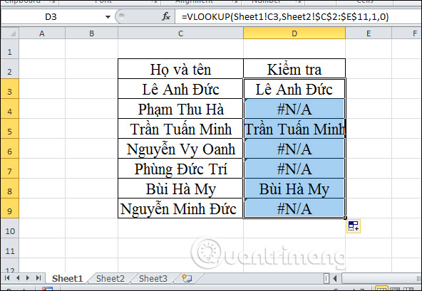
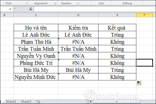
The final result will show the name of the duplicated person.

How to filter duplicate data on 2 Excel sheets Picture 9

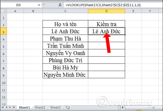
Continue dragging the data in the first cell to the remaining cells. Since the area has been fixed, the function will not be roamed when copying the function formula. For cells that do not have the same data will return the # N / A error.

How to filter duplicate data on 2 Excel sheets Picture 10

Step 5:

So we know in detail how to enter the Vlookup formula with each element in the recipe. To shorten the way, enter the formula like below.

1. = VLOOKUP (Sheet1! C3, Sheet2! $ C $ 2: $ E $ 11.1,0)

How to filter duplicate data on 2 Excel sheets Picture 11

Inside:

1. Sheet1! C3 is cell C3 in Sheet 1, it is necessary to check the duplicate data.
2. Sheet2! $ C $ 2: $ E $ 11 is the same data area to check in Sheet 2.
3. 1 is the column where you want thelook function to return in the data area to be checked.
4. 0 is the exact search type of Vlookup function.

2. Combining Vlook function, If function, ISNA function removes # N / A error

In the data check column for those cells that are not duplicated, the # N / A error will be displayed. If so, it can be combined with ISNA function to help you check the data # N / A. If the data is # N / A, the ISNA function will return TRUE, otherwise the function will return FALSE.

If the function checks the condition, it returns the value you specified, if it is false, returns the b value that the user specifies.

Step 1:

At Sheet 1 you enter 1 more column to compare with the Check column. In the first box you will enter the formula below.

1. = IF (ISNA (VLOOKUP (Sheet1! C3, Sheet2! $ C $ 2: $ E $ 11,1,0)), "No", "Duplicate")

ISNA function will check the value of Vlookup function. If Vlookup function returns the # N / A error, the ISNA function will return TRUE value. Where # N / A is a non-duplicate data, If will return the result No.

If VLOOKUP returns a specific value, the ISNA function will return FALSE. The IF function will return a false condition of 'Duplicate'.

How to filter duplicate data on 2 Excel sheets Picture 12

Step 2:

The results in the first box will notify the same. Continuing to scroll down to the boxes below will get different messages, corresponding to each value.

How to filter duplicate data on 2 Excel sheets Picture 13

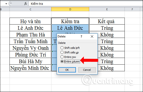
Step 3:

So you have the results of the Notification and No notification for the checklist. Finally, we can delete the Check column to compact the data table and interface more scientific tables without the # N / A error message.

How to filter duplicate data on 2 Excel sheets Picture 14

Results of complete Sheet 1 data sheet as shown.

How to filter duplicate data on 2 Excel sheets Picture 15

Above is how to use Vlookup function to search for duplicate values ​​from multiple sheets on Excel. If done, you should combine the ISNA function, IF function and VLOOKUP function to produce more beautiful and faster filter results.

See more:

1. How to copy Word data to Excel keeps formatting
2. Instructions on how to separate column content in Excel
3. How to rank on Excel with RANK function

I wish you all success!