Use VLOOKUP to join two Excel tables together

In Excel, you can merge rows from this table into another table by copying and pasting them into the first blank below the table. And if the rows match, you can merge columns from one table to another by pasting them into the first blank on the right of the table.

Connecting rows is quite simple, but linking columns of this table to another table is more complicated because the rows in this table do not always correspond to the other table. By using VLOOKUP to join the table you will avoid these annoying sorting problems.

In the example below, we have 2 tables, Blue and Orange. In the Blue table, each row is a detailed item in the order. Order ID 20050 has 2 items, Order ID 20051 has 1 item, Order ID 20052 has 3 items, so on until the end of the table. Now we need to merge the Sales ID and Region ID columns into the Blue table, based on the appropriate values ​​in the Order ID column of the Orange table.

But the Order ID value is repeated in the Blue table, while the Orange Order ID is unique. So if you are innocent but Ctrl + C then Ctrl + V to paste, you will notice the mess in the spreadsheet. If the data is too much, you will be crazy about having to rearrange them. Try VLOOKUP and see the difference.

Here are two spreadsheets, you can copy into Excel file to follow if desired. Copy these two tables into the same Excel page, press Ctrl + T to turn it into a spreadsheet, name the worksheet in Table name, Blue and Orange respectively.

Blue board:

20050

2/2/14

C6077B

20050

2/2/14

C9250LB

20051

2/2/14

M115A

20052

2/3/14

A760G

20052

2/3/14

E3331

20052

2/3/14

SP1447

20053

2/3/14

L88M

20054

April 2, 14

S1018MM

20055

2/5/14

C6077B

20056

June 2, 14

E3331

20056

June 2, 14

D534X

Orange Table:

20050

447

West

20051

398

South

20052

1006

North

20053

447

West

20054

885

East

20055

398

South

20056

644

East

20057

1270

East

20058

885

East

Then, copy the Sales ID and Region header next to the Product ID header in the Blue table. Now your spreadsheet will look like this:

Use VLOOKUP to join two Excel tables together Picture 1

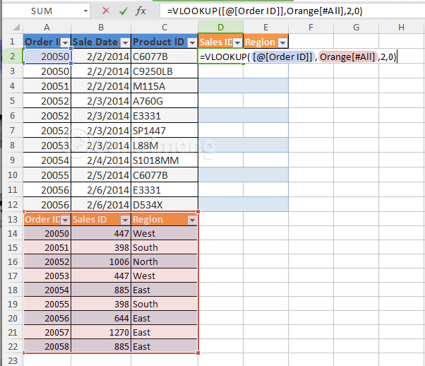
In cell D2, enter the following formula:

 =VLOOKUP([@[Order ID]],Orange[#All],2,0) 

1. The [@ [Order ID]] section means "get the value in this row from the Order ID column".
2. The "Orange [#All]" parameter can be entered manually if you have named the table, otherwise, simply highlight the entire Orange table with your mouse to get the function automatically and then add $ in front, or enter $ A $ 13: $ C $ 22 to select the Orange table.
3. 2 is the serial number of the Sales ID column in the Orange table.
4. 0 is relative detection (because here the Order ID of both tables are sorted, otherwise you must use absolute detection, replacing 0 with 1).

Use VLOOKUP to join two Excel tables together Picture 2

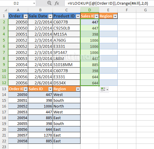
Then the result returned in cell D2 will be 447.

Use VLOOKUP to join two Excel tables together Picture 3

Click on the lower right corner of cell D2 until the plus sign appears, drag the mouse down to the end of the Blue table, you will get the following result:

Use VLOOKUP to join two Excel tables together Picture 4

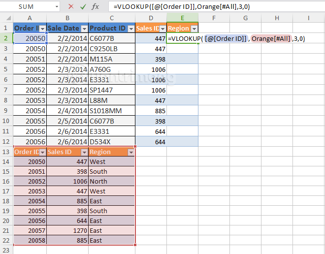
To enter the Region column into the Blue table, simply copy the formula in cell D2 into cell E2, edit the third parameter from 2 to 3, to indicate that you want to get the third column (Region) of the Orange table.

Use VLOOKUP to join two Excel tables together Picture 5

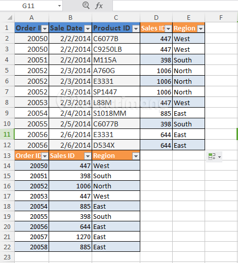
Then point to the lower right corner of cell E2 until the plus sign appears, drag the mouse down to the end of the Blue table, you will get the following result:

Use VLOOKUP to join two Excel tables together Picture 6

As you have seen with using VLOOKUP to pair two Excel tables the data will be correctly populated, the operation is not too complicated, just a few clicks are done. This is an Excel sample file, if you still find it confusing, download it to see it for visualization.

Hopefully the trick with this VLOOKUP function is useful to you.

See also: How to use SUM in Excel