Vlookup Function in Excel: Syntax, Examples, and Tips

This article provides a clear overview of Vlookup Function in Excel, with the main facts, useful context, and practical details organized for easy reading.

Description

The Vlookup function is a column lookup function, which searches for a value in the first column from the left of the data table. If the function is found, it will return one of the next columns in the same row as the value in the first column you specify.

The function is usually used to fill information into the main table with data taken from the secondary table.

The Syntax of the Vlookup Function

= VLOOKUP (lookup_value, table_array, col_index_num, range_lookup)

Arguments

- lookup_value: value to search, this value can be a string, a reference or some value of the main table. If the lookup_value value is smaller than the smallest value in the first column of the table_array sub-table, the Vlookup function returns the error value.

- table_array: reference table or table containing the values to search, the values in the first column of table_array are the values searched by lookup_value. This value can be text, number or logical value.

- col_index_num: index column in table_array will get the value returned to the main table. If col_index_num value is less than 1 or greater than the number of columns in table_array, the function will return an error value.

- range_lookup: is a logical value that helps you specify the Vlookup function to find exact or relative searches.

+ If range_lookup is TRUE or omitted, the function will relatively detect the values in the first column in table_array must be arranged in order to avoid Vlookup function returning incorrect values.

+ If range_lookup is FALSE value, the function searches exactly the values in the first column in table_array without any sort order.

For Example:

- Detect Relative.

The following data sheet is available, please fill in the HK Class and Symbol information based on the Class table information.

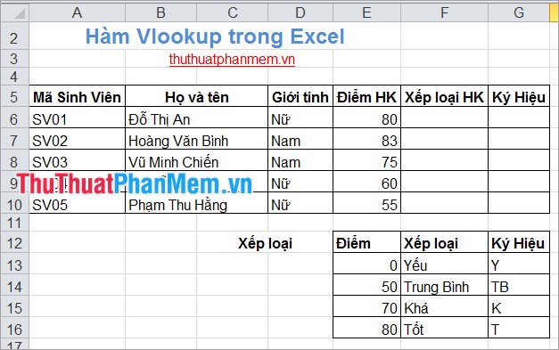
- Fill information for the HKType column, how to enter the formula as follows:

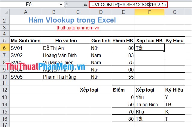
First, select the mouse in the SV Ranking box of SV01, enter the formula as follows: you enter = VLOOKUP (E6, then you use the mouse to select (black out) the Sort sub-table, then release the mouse button and press the next F4 key you enter, 2,1).

The formula you get is as follows: = VLOOKUP (E6, $ E $ 12: $ G $ 16,2,1).

Arguments

E6 is the value to be searched (above example is 80).

$ E $ 12: $ G $ 16 is the table of values to be searched (the above example is the Ranking table).

2 is column 2 in the table of information values to be searched, the data of column 2 will be filled in the main table (the above example is the HK Rank column in the Ranking table).

1 is relative detection.

- Enter the information for the Symbol column, you enter the same formula as the HK Rank column but the col_index_num value in VLookup you choose is 3, corresponding to the column will be taken the value in the Sort column as Symbol column.

= VLOOKUP (E6, $ E $ 12: $ G $ 16,3,1)

- Absolute detection (correct) you only need to change the range_lookup value to 0 or FALSE , but if the lookup_value value is not found in the first column of the secondary reference table, the function will report an error.

With this simple example, I hope you will understand how to use Vlookup function in Excel. Depending on the actual requirements, you can use the Vlookup function to process data on Excel spreadsheets. Good luck!