Filter data in Excel with Advanced Filter

In the process of working with data tables in Excel, the filtering of data in the data tables is very necessary and often done. There are many ways to filter and functions to help you filter data in data tables.

Advanced Filter function is one of the functions that help you filter data, Advanced Filter does not limit the filtering conditions, so it will help you filter data faster and more efficiently.

The following article will guide how to use the Advanced Filter function to filter data in Excel.

Required when using the Advanced Filter

To use the Advanced Filter function, the data table to filter needs to meet the following requirements:

- Data sheet header must use only one line.

- Do not merge any cells in the data table to filter.

- Leave at least 3 lines in the same table.

For example, we have the following data table:

To use the Advanced Filter function, you need a filter condition table.

Create filter conditions table

How to create filter conditions as follows:

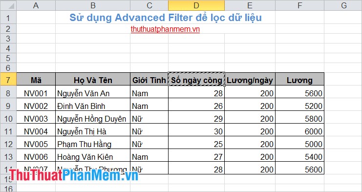
Step 1: Select the column header to be filtered, then select Home -> Copy (or Ctrl + C ).

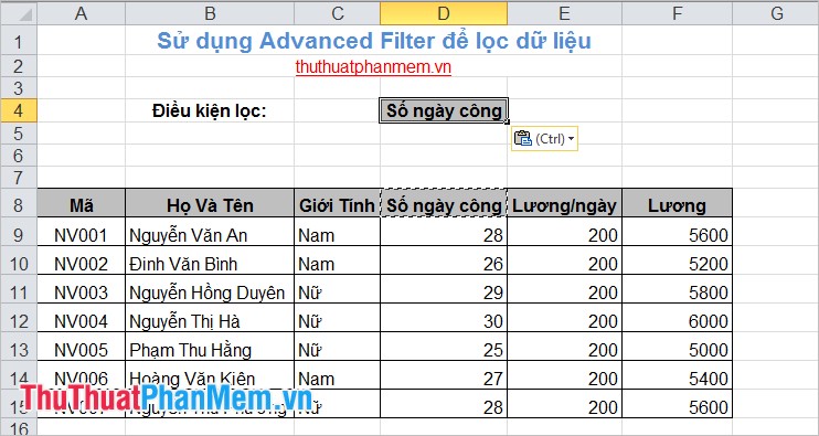
Step 2: Paste ( Ctrl + V ) into any cell in Excel.

Step 3: Enter filtering conditions.

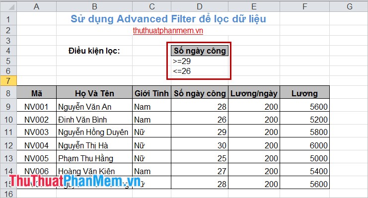
- OR conditions are arranged vertically. For example:

Number of workdays <= 26 or number of workdays> = 29.

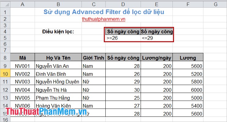
- AND conditions are arranged in horizontal rows, so if you need to filter 2 AND conditions under the same criteria, you must use a title for 2 cells. Examples of AND conditions:

Number of workdays> = 26 and <= 29.

Number of workdays> 2 = 28 and Gender is Male.

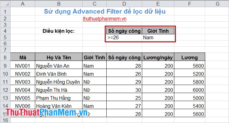
- With only one condition, you only need to enter it under the title box of the filter table.

- Also you can combine AND and OR conditions together.

After creating filter conditions, you start using the Advanced Filter function to filter data.

Use the Advanced Filter function

Step 1: Select Data -> Advanced .

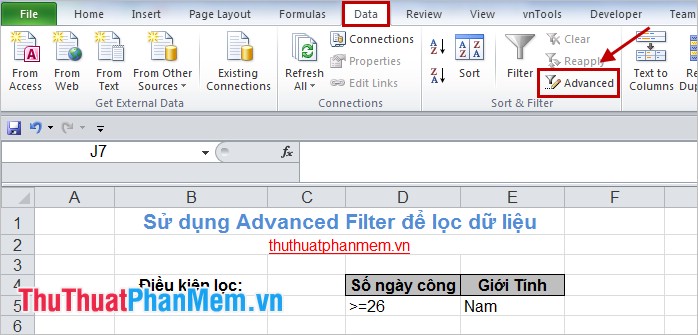
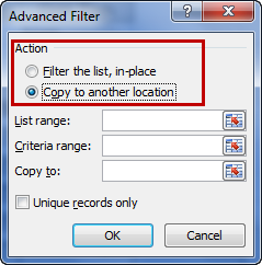
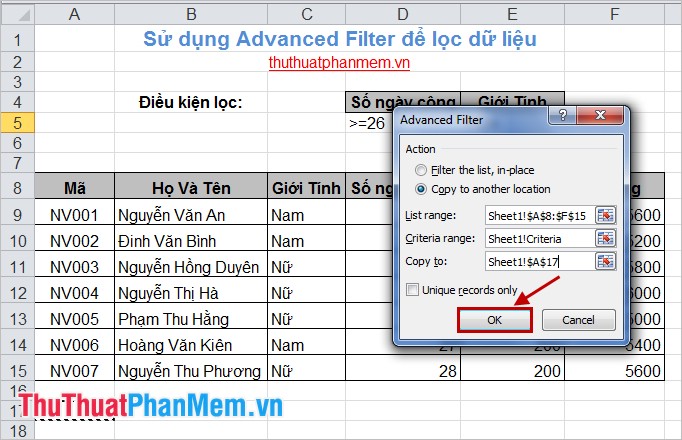
Step 2: The Advanced Filter dialog box appears , in the Action section there are 2 options:

- Filter the list, in-place: filter and return results in the filter data table itself.

- Copy to another location: filter and return filter results in other locations, you choose.

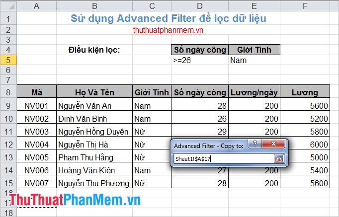
For example, select Copy to another location .

Step 3: In the List range section , click the icon at the end of the line as shown below:

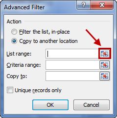
Then you click to select the main data table to be filtered by clicking, holding and dragging to the last cell in the table.

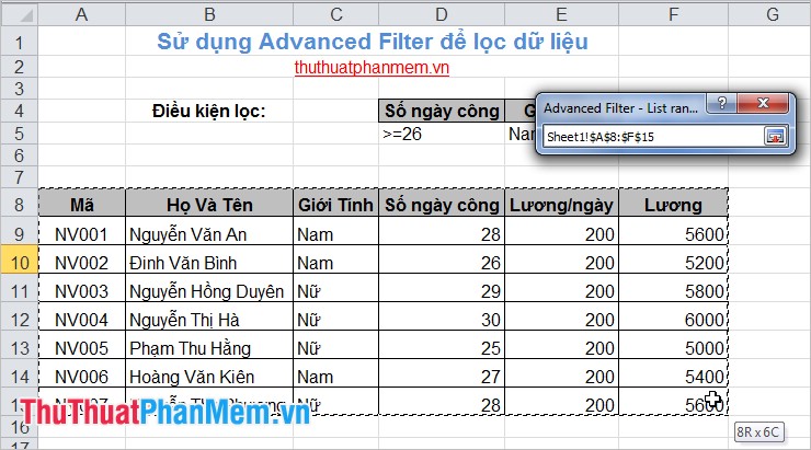
Release the mouse button and click the icon as shown below to return to the Advanced Filter dialog box .

Step 4: In the Criteria range section , you also do the same to select the filter condition table.

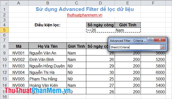
Step 5: Because of selecting Copy to another location , you need to select the box in the Copy to section .

Then you click OK .

The final result after filtering:

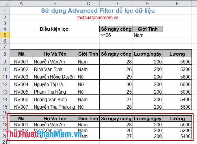
Advanced Filter function can combine many different conditions, the processing of data in your Excel spreadsheet will be easier. Good luck!