How to Filter Data in Excel: Step-by-Step Guide

This updated guide explains how to Filter Data in Excel through clear steps, practical examples, and important checks that help prevent common errors.

this guide will guide how to filter data in an Excel table:

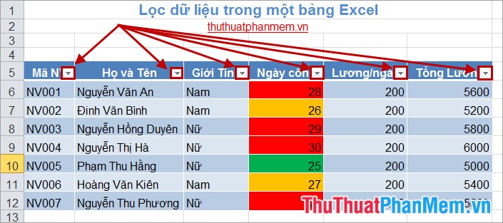
When you create a table in Excel, on the column headings in the table will automatically add filter controls.

Filter Fast

Step 1: You choose the triangle icon in the column header to filter data.

Step 2: In the dialog box that appears, uncheck the box before Select All . Next you may need to filter the data by which item in the column you tick the square before that data. Then click OK .

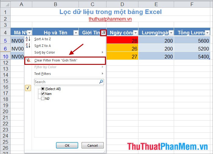
The result will filter all the data as you choose, and the title of the filtered column will appear as a filter icon.

To remove the filter, select the filter icon at the top of the column header and select -> Clear Filter From "column heading".

Filter by Specific Text or Number

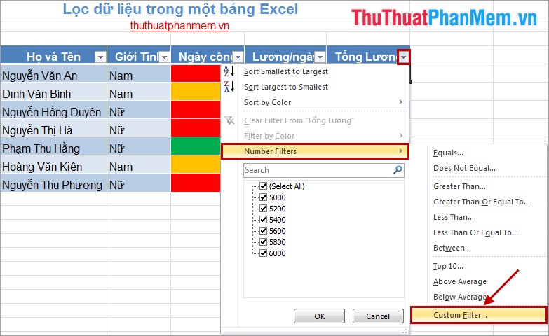
Step 1: Select the triangle icon in the cell where you may need to filter the data.

Step 2: If the data column contains text to filter, you select Text Filters , if the data column contains numbers to filter, select Number Filters . Then select Custom Filter .

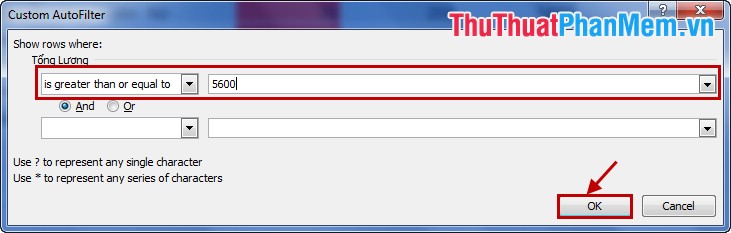
Step 3: In the dialog box Custom AutoFilter , you enter the filter condition if there are 2 filter conditions you enter both conditions into the data cells. Choose the relationship between And and Or conditions to match the filter condition. Then click OK .

Example

Filter data provided that Total Wage is greater than or equal to 5600.

Results after filtering:

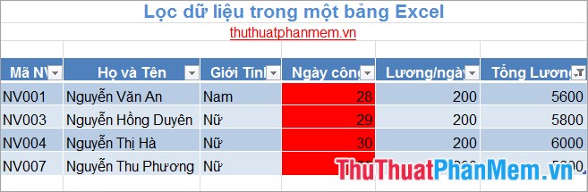
Filter Items by Color

If during the process of entering data in the table, you marked the data cells with different colors. You can filter data by the following colors:

Step 1: Select the filter icon in the header cell of the color-formatted column.

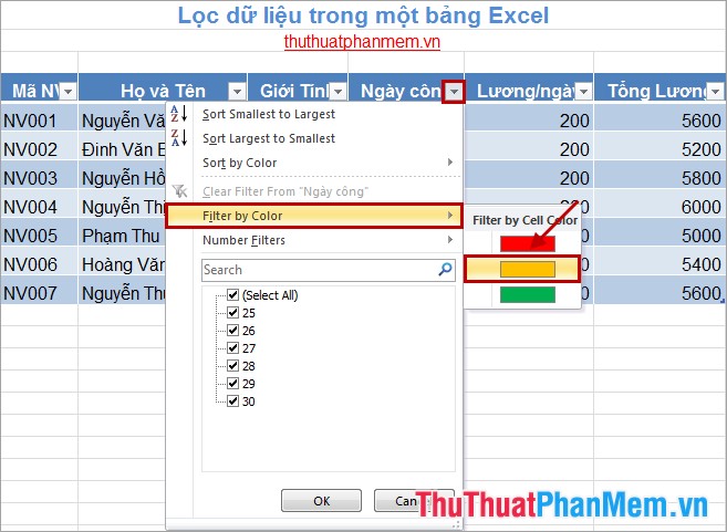
Step 2: Select Filter by Color then select the color you may need to filter.

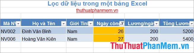
Results after you filter by color:

Also in Excel 2013 you can create slicers to filter your table data.

Step 1: You select any cell in the table, select the Design tab of Table Tools -> Insert Slicer .

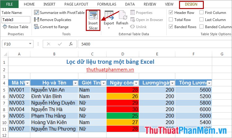
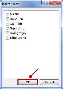
Step 2: Next in the dialog box Insert Slicers you select the columns to filter data and click OK .

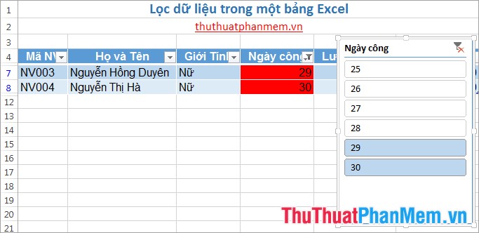
Step 3: The dialog box containing the column you selected above appears, you select the data in the dialog boxes (if you select multiple columns to filter). Hold down Ctrl to select multiple data in a column. Thus the data in the table will quickly be filtered according to your requests.

With the ways of filtering data in the above Excel table, managing the data in your tables will no longer be complicated. Good luck!