How to compare data on 2 different sheets in Excel file

To compare data on 2 different sheets but in the same Excel file, we have many different methods such as using VLOOKUP or using the COUNTIF function and combining with Conditional Formating to create different comparison effects. or no difference in data in two different sheets. But in this article of TipsMake.com, we will use COUNTIF and Conditional Formating methods to compare data.

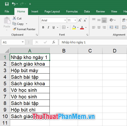
First of all we have a column of data as follows in Sheet 1. It is a list of items on stock on day 1.

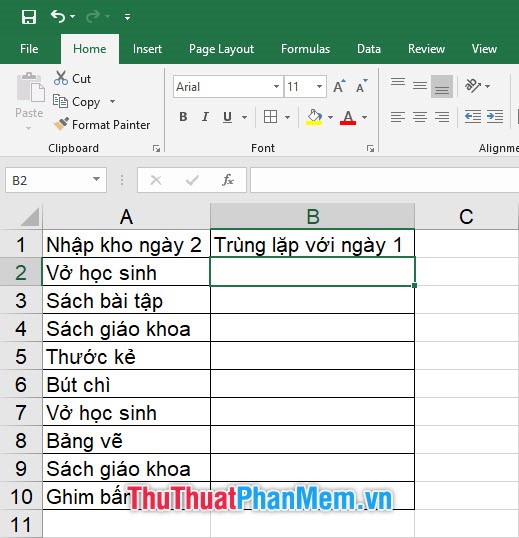
And on sheet two, we have a list of items to stock on day 2. Now we can use the COUNTIF function to calculate the number of duplicates of items compared to the first day.

Before you start writing the formula you need to limit the data to be compared in sheet 1 and give it a distinguished name.

Highlight the data range to select and then click on the name of the cell in the left corner of the sheet, enter a name for the range. The name you enter must be spaces without Excel or Excel will not be able to read the name of the data range.

Or you can also name the area by going to the Formulas ribbon on the toolbar and selecting Define Name in the Defined Names section .

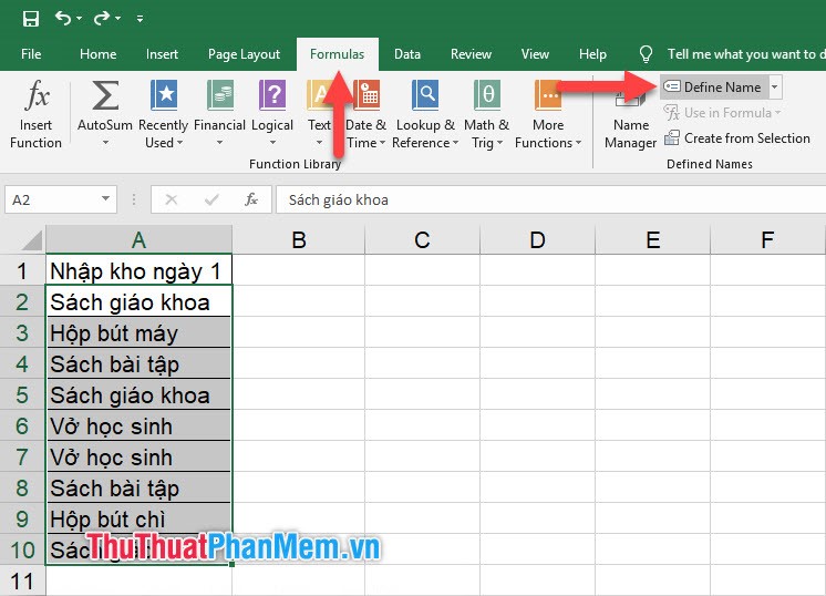
Enter a name for the range in the Name box, then click OK to confirm the name.

Now that your data range in Sheet 1 has a custom name, you can call that range in a formula without having to write an address sign. This method is very convenient for using data on many different sheets.

The COUNTIF formula we need to use here to count duplicates for those two data columns is:

= COUNTIF (array of data to be counted, different conditions to count)

And for the example in the image, we have the function formula:

= COUNTIF (input1; A2)

With this formula we can count the number of times "School notebooks" appear in the first day of inventory data.

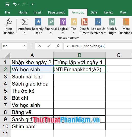
Next, you just need to copy the formula down by clicking on the lower right corner of the available formula box and dragging the mouse down.

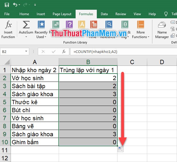
As you will see a zero result shows that this item was never stocked in the first day.

The above steps can show you the specific number of items in the duplicated inventory but do not show the duplication right on the data column. We can do this by using the Conditional Formating function , creating a different format so that we can immediately see which item is the item without duplication when compared to the inventory data. first.

Highlight the array to compare, then go to the Home ribbon on the toolbar and select Conditional Formating located in the Styles section of this ribbon.

Click on the New Rule line .

Then the New Formatting Rule function dialog box will appear, select the last line of the list of rule types is Use a formula to determine which cells to format .

In the Format values ​​where this formula is true box (format the cells with the following formula), enter the following formula:

= B2 = 0

To explain a bit for this. Because we need to color data cells without duplicates, it means that in that data line the result in the " Duplicate with Day 1 " column we just filled out with the COUNTIF formula is 0.

So when we fill in the condition for this cell, we need to include the condition that finds the zero cells in that " Duplicate with Day 1 " column .

You leave B2 as a non-fixed parameter cell so that it can be modified with every row in the column.

Then don't forget to change the format for the cell with the appropriate condition by going to Format .

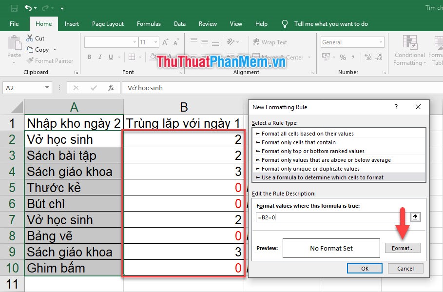
Change the format of the cell to suit the conditions in the different tabs of the Format Cells dialog box , with Font being the font change, Border to change the border of the cell and Fill to fill the background color for that data cell. Then click OK to confirm.

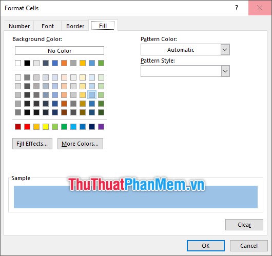
After looking at a series of settings, click OK to start changing the format for the cells matching the conditions set.

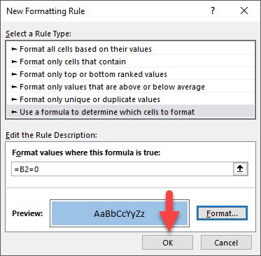
As you will see, the boxes that match the conditions set out are items that do not coincide with the first day of storage will be colored blue on your box.

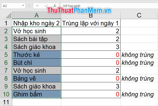
If you want to directly change the format for cells with non-duplicated data, you can use the Excel COUNTIF formula directly into the Format values ​​where this formula is true .

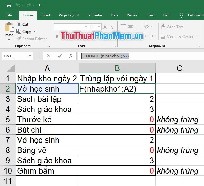
From there, we have the formula for Format values ​​where this formula is true :

= COUNTIF (input1; A2) = 0

And the results received:

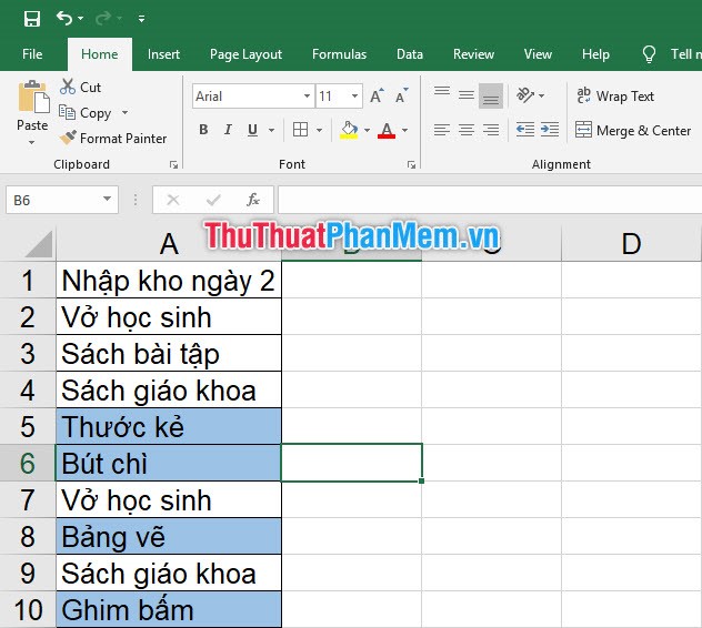
Note: If you change the formula from = 0 to> 0, the cells with duplicate data from the first date will have a format change. This part, TipsMake.com will leave you guys to try it out.

The article about how to compare data on 2 different sheets of Dexterity Software is here, thank you for following our article. Hope you can understand the knowledge we want to impart and successfully implement it for our data.