How to Highlight Duplicate Data in Google Sheets

HOW TO HIGHLIGHT DUPLICATE CONTENT

This works by color coding duplicates so you can easily check them. This formula is the simplest and most effective.

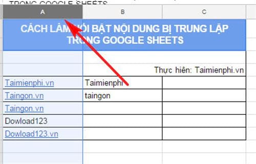
Step 1 : Open the spreadsheet

Step 2 : Select the column you want to highlight

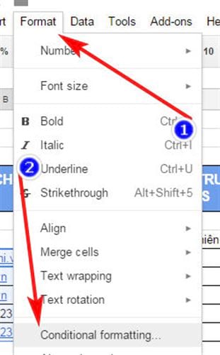
Step 3 : Select Format on the toolbar and then select Conditional Formatting

Step 4 : In the Apply to range section , the data column you selected above will be automatically added.

Step 5 : In ' Format cells if' we change the value here to 'Custom formula is'

Step 6 : Enter the following in the box below: '=countif(A:A,A1)>1'

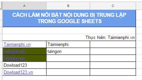
Step 7 : In the Formatting Style section , you can change the color to fill the cells. Here I choose red. Then click Done to complete.

Now the duplicate data will be highlighted in red immediately. Now you can check again if this data needs to be deleted or not.

Coloring duplicate data in Google Sheets makes managing your spreadsheets easier. Use Conditional Formatting or the COUNTIF function to handle data accurately.

David Pac

Update 14 March 2025