In Excel file, you have data in 2 different sheets but you want to filter duplicate data with a large number of records. So, let's follow the article below to know how to filter duplicate data from 2 sheets in Excel.

How to filter duplicate data from 2 Sheets in Excel Picture 1

Here's how to use the VLOOKUP function to filter duplicate data from 2 Sheets in Excel, please follow along.

Use the VLOOKUP function to filter duplicate data in 2 sheets

Suppose you have the following Sheet 1 data:

How to filter duplicate data from 2 Sheets in Excel Picture 2

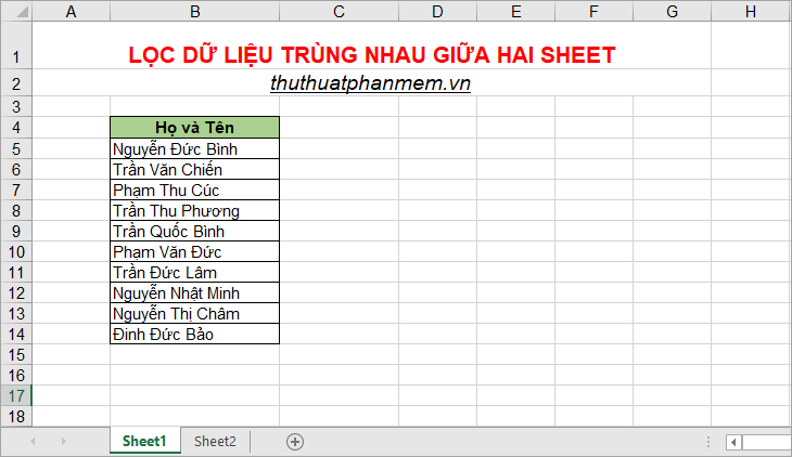
Sheet 2 data as follows:

How to filter duplicate data from 2 Sheets in Excel Picture 3

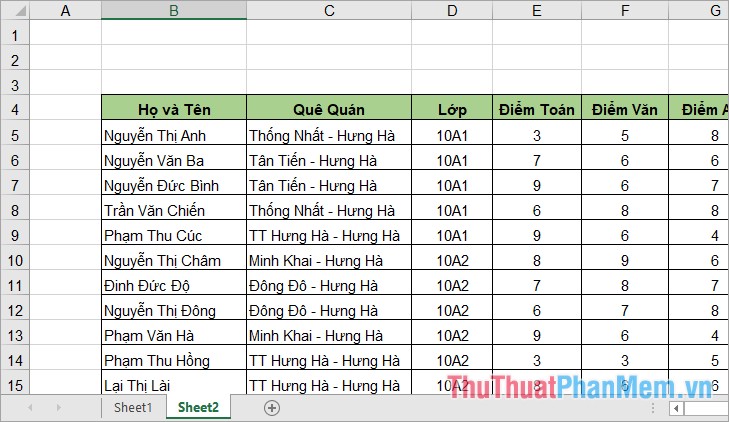
To check for duplicate data, enter the Vlookup function formula in the first cell as follows:

= VLOOKUP (Sheet1! B5; Sheet2! $ B $ 4: $ G $ 33; 1; 0)

Where: Sheet1! B5 is cell B5 in Sheet1 to check for duplicate data.

Sheet2! $ B $ 4: $ G $ 33 is the data area to check for duplicate data in Sheet 2.

1 is the column you want the Vlookup function to return in the data area to be checked.

0 is the exact lookup type for the Vlookup function.

If you are not familiar with the Vlookup function, you can see more articles on how to use this Vlookup function ++++++++ ________________ +++++++++++++++++++

Thus, if the data is duplicated, the function will return the same data.If the data does not match, the function will return the # N / A error.

How to filter duplicate data from 2 Sheets in Excel Picture 4

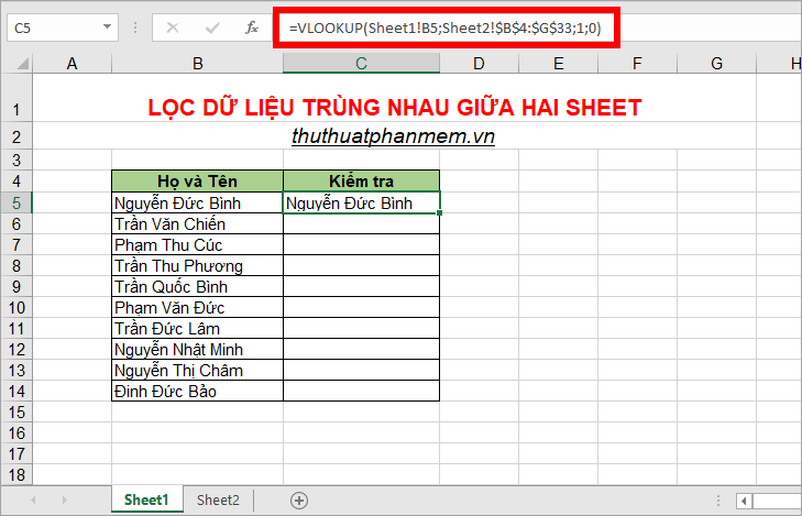
How to write the Vlookup function

Vlookup function with data from two sheets should have the sheet name before each value, you can enter the function as usual. If you are more careful, you can write Vlookup function as follows:

1. Select the mouse in cell C5 of Sheet 1 (the first cell to check for duplicate data), next you choose Formulas tab -> Insert Function.

How to filter duplicate data from 2 Sheets in Excel Picture 5

2. The Insert Function dialog box that you select in the Or select a category (1) is Lookup & Reference because Vlookup belongs to this group, so select it in the Select a function section to shorten the search to the function. Vlookup more. Next select Vlookup in the Select a function (2) section and select OK .

How to filter duplicate data from 2 Sheets in Excel Picture 6

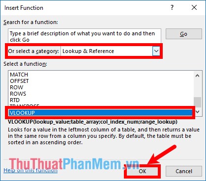
3. The Function Arguments dialog box appears, you will see the arguments in the Vlookup function, where you select the data in turn for the arguments as follows:

1. In the Lookup_value section , place your cursor here then select cell B5 in Sheet 1, this time in Lookup_value will appear Sheet1! B5.

How to filter duplicate data from 2 Sheets in Excel Picture 7

1. Next in the Table_array section, place your cursor in this section and select sheet 2 and select the data area to check for duplicate data. So in Table_array will appear Sheet2! B4: G33 with B4: G33 is the area you choose.

How to filter duplicate data from 2 Sheets in Excel Picture 8

1. If you want to check a lot of data, you need to fix this selection by placing the cursor in the middle or the bottom of the B4 press the F4 key , then the mouse at the end of the G33 and press the F4 key to position. So now Table_array will be Sheet2! $ B $ 4: $ G $ 33 as shown below.

How to filter duplicate data from 2 Sheets in Excel Picture 9

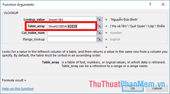
1. Next in the section Col_index_num you enter the position of the column that you want to return data if the two data are the same, for example if the data is the same, you return the same data, then you enter the number 1 to returns the corresponding data in the first column. In the Range_lookup section you enter 0 for the exact search function. Then click OK to add the function to the cell you select.

How to filter duplicate data from 2 Sheets in Excel Picture 10

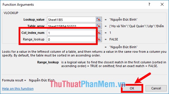
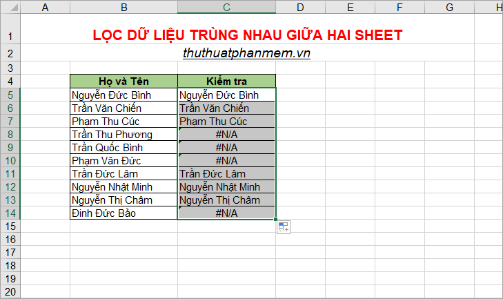
So you will get the following results:

How to filter duplicate data from 2 Sheets in Excel Picture 11

To check the data below, you only need to copy the formula, because you have fixed the area, the function will not be roamed when you copy the formula. Your results will return duplicate data, non-duplicate data will return the # N / A error.

How to filter duplicate data from 2 Sheets in Excel Picture 12

Combine the IF and ISNA functions to eliminate the # N / A error

ISNA function helps you check the # N / A data, if the data is # N / A, the ISNA function will return TRUE, otherwise it will return FALSE.

The IF function helps you check if the condition is true, the function will return the value you specified, if the condition is false, the function will return the value b you specify.

So with the above example, instead of just using the Vlookup function, you can combine the IF function and the ISNA function to check the data, enter the following formula:

= IF (ISNA (VLOOKUP (Sheet1! B5; Sheet2! $ B $ 4: $ G $ 33; 1; 0)); "No"; "Duplicate data")

The ISNA function checks the return value of the VLOOKUP function, if VLOOKUP returns the # N / A value, the ISNA function will return TRUE. Which VLOOKUP returns # N / A if the data is not duplicated. So the IF function will return 'No'.

If the VLOOKUP function returns a specific value, the ISNA function will return the FALSE value and the IF function will return the false condition of 'Duplicate data'.

How to filter duplicate data from 2 Sheets in Excel Picture 13

Similarly, you copy the formula down the line below and get the following result:

How to filter duplicate data from 2 Sheets in Excel Picture 14

Above the article has shared to you how to filter duplicate data from 2 sheets in Excel. This way you can quickly filter duplicates between different sheets. Hope this article will help you. Good luck!